梯度提升方法(Gradient Boosting)算法案例

GradientBoost算法 python实现，该系列文章主要是对《统计学习方法》的实现。

完整的笔记和代码以上传到Github,地址为（觉得有用的话，欢迎Fork,请给作者个Star）：

https://github.com/Vambooo/lihang-dl

提升树利用加法模型与前向分步算法实现学习的优化过程，当损失函数为平方损失和指数损失函数时，每一步优化都较为简单。但对一般损失函数来说，每一步的优化并不容易。Fredman为了解决这一问题，便提出了梯度提升(Gradient Boosting)方法。

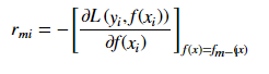
梯度提升法利用最速下降的近似方法，这里的关键是利用损失函数的负梯度在当前模型的值r_{mi}作为回归问题提升树算法中的残差的近似值，拟合一个回归树。

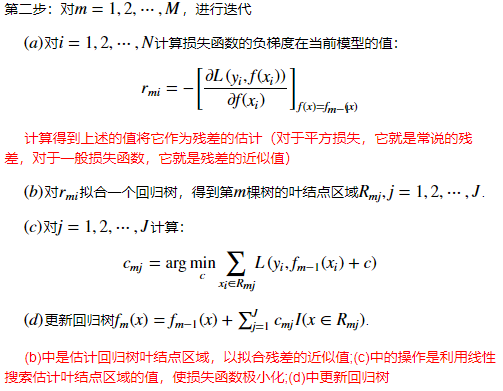
梯度提升方法(Gradient Boosting)算法

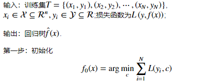
注：该步通过估计使损失函数极小化的常数值，得到一个根结点的树。

Gradient Boost算法案例 python实现(马疝病数据)

(代码可以左右滑动看)

import pandas as pdimport numpy as npimport matplotlib.pyplot as pltfrom sklearn import ensemblefrom sklearn import linear_model

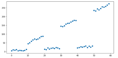
第一步：构建数据

# 创建模拟数据xx = np.arange(0, 60)y=[ x / 2 + (x // 10) % 2 * 20 * x / 5 + np.random.random() * 10 for x in xx]
x = pd.DataFrame({'x': x})
# Plot mock dataplt.figure(figsize=(10, 5))plt.scatter(x, y)plt.show()

线性回归模型来拟合数据

linear_regressor = linear_model.LinearRegression()linear_regressor.fit(x, y)
plt.figure(figsize=(10, 5))plt.title("Linear Regression")plt.scatter(x, y)plt.plot(x, linear_regressor.predict(x), color='r')plt.show()

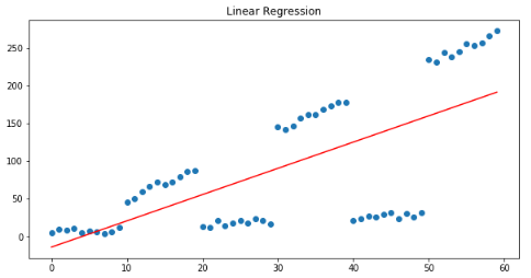
线性回归模型旨在将预测与实际产出之间的平方误差最小化，从我们的残差模式可以清楚地看出，残差之和约为0：

梯度提升法使用一组串联的决策树来预测y

下面从只有一个估计量的梯度提升回归模型和一个只有深度为1的树开始：

params = {    'n_estimators': 1,    'max_depth': 1,    'learning_rate': 1,    'criterion': 'mse'}
gradient_boosting_regressor = ensemble.GradientBoostingRegressor(**params)
gradient_boosting_regressor.fit(x, y)
plt.figure(figsize=(10, 5))plt.title('Gradient Boosting model (1 estimators, Single tree split)')plt.scatter(x, y)plt.plot(x, gradient_boosting_regressor.predict(x), color='r')plt.show()

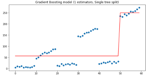
从上图可以看到深度1决策树在x<50  和x>50处被拆分，其中：

if x<50 ,y=56;

if x>=50,y=250.

这样的拆分结果肯定是不好的，下面用一个估计量时，30-40之间的残差很。猜想：如果使用两个估计量，把第一棵树的残差输入下一棵树中，有怎样的效果？验证代码如下：

params['n_estimators'] = 2
gradient_boosting_regressor = ensemble.GradientBoostingRegressor(**params)
gradient_boosting_regressor.fit(x, y)
plt.figure(figsize=(10, 5))plt.title('Gradient Boosting model (1 estimators, Single tree split)')plt.scatter(x, y)plt.plot(x, gradient_boosting_regressor.predict(x), color='r')plt.show()

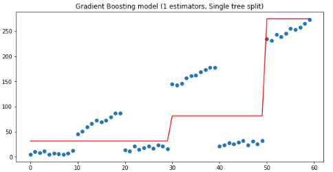
如上图，当有连个估计量时，第二棵树是在30处拆分的，如果我们继续增加估计量，我们得到Y分布的一个越来越接近的近似值：

f, ax = plt.subplots(2, 2, figsize=(15, 10))
for idx, n_estimators in enumerate([5, 10, 20, 50]):    params['n_estimators'] = n_estimators
    gradient_boosting_regressor = ensemble.GradientBoostingRegressor(**params)
    gradient_boosting_regressor.fit(x, y)    subplot = ax[idx // 2][idx % 2]    subplot.set_title('Gradient Boosting model ({} estimators, Single tree split)'.format(n_estimators))    subplot.scatter(x, y)    subplot.plot(x, gradient_boosting_regressor.predict(x), color='r')plt.show()

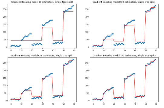
上面是改变估计量，保持树深度的效果，下面保持估计量为10，改变树的深度.

params['n_estimators'] = 10
f, ax = plt.subplots(2, 2, figsize=(15, 10))
for idx, max_depth in enumerate([1, 2, 3, 5]):    params['max_depth'] = max_depth
    gradient_boosting_regressor = ensemble.GradientBoostingRegressor(**params)
    gradient_boosting_regressor.fit(x, y)    subplot = ax[idx // 2][idx % 2]    subplot.set_title('Gradient Boosting model (10 estimators, {} max tree splits)'.format(max_depth))    subplot.scatter(x, y)    subplot.plot(x, gradient_boosting_regressor.predict(x), color='r')plt.show()

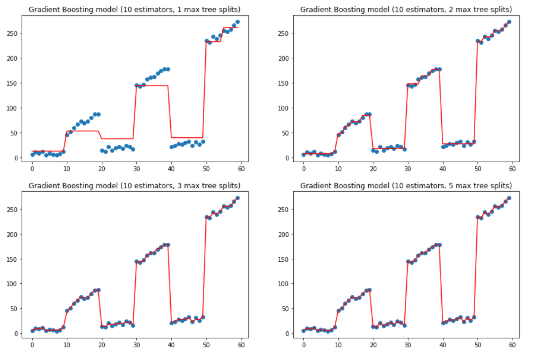
上两图可以看到如何通过增加估计量和最大深度来拟合y值。不过有点过拟合了。