

关于激光雷达传感器如何投影成二维图像
描述
“前视图”投影
为了将激光雷达传感器的“前视图”展平为2D图像,必须将3D空间中的点投影到可以展开的圆柱形表面上,以形成平面。
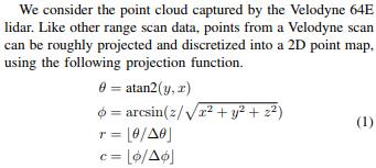
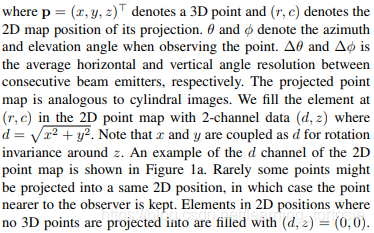
问题在于这样做会将图像的接缝直接放在汽车的右侧。将接缝定位在汽车的最后部更有意义,因此前部和侧部更重要的区域是不间断的。让这些重要区域不间断将使卷积神经网络更容易识别那些重要区域中的整个对象。
以下代码解决了这个问题。
沿每个轴配置刻度
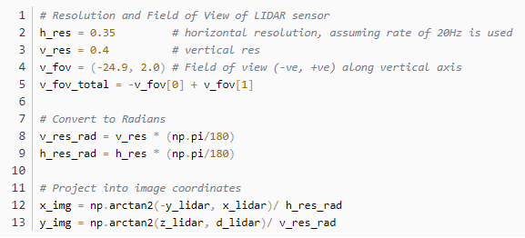
变量h r e s h_{res}和v r e s v_{res}非常依赖于所使用的LIDAR传感器。在KTTI数据集中,使用的传感器是Velodyne HDL 64E。根据Velodyne HDL 64E的规格表,它具有以下重要特征:
垂直视野为26.9度,分辨率为0.4度,垂直视野被分为传感器上方+2度,传感器下方-24.9度
360度的水平视野,分辨率为0.08-0.35(取决于旋转速度)
旋转速率可以选择在5-20Hz之间
可以按以下方式更新代码:
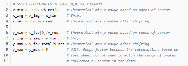
然而,这导致大约一半的点在x轴负方向上,并且大多数在y轴负方向上。为了投影到2D图像,需要将最小值设置为(0,0),所以需要做一些改变:
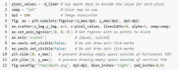
绘制二维图像
将3D点投影到2D坐标点,最小值为(0,0),可以将这些点数据绘制成2D图像。
完整代码
把上面所有的代码放在一个函数中。
def lidar_to_2d_front_view(points, v_res, h_res, v_fov, val=“depth”, cmap=“jet”, saveto=None, y_fudge=0.0 ): “”“ Takes points in 3D space from LIDAR data and projects them to a 2D ”front view“ image, and saves that image.
Args: points: (np array) The numpy array containing the lidar points. The shape should be Nx4 - Where N is the number of points, and - each point is specified by 4 values (x, y, z, reflectance) v_res: (float) vertical resolution of the lidar sensor used. h_res: (float) horizontal resolution of the lidar sensor used. v_fov: (tuple of two floats) (minimum_negative_angle, max_positive_angle) val: (str) What value to use to encode the points that get plotted. One of {”depth“, ”height“, ”reflectance“} cmap: (str) Color map to use to color code the `val` values. NOTE: Must be a value accepted by matplotlib‘s scatter function Examples: ”jet“, ”gray“ saveto: (str or None) If a string is provided, it saves the image as this filename. If None, then it just shows the image. y_fudge: (float) A hacky fudge factor to use if the theoretical calculations of vertical range do not match the actual data.
For a Velodyne HDL 64E, set this value to 5. ”“”
# DUMMY PROOFING assert len(v_fov) ==2, “v_fov must be list/tuple of length 2” assert v_fov[0] 《= 0, “first element in v_fov must be 0 or negative” assert val in {“depth”, “height”, “reflectance”}, ’val must be one of {“depth”, “height”, “reflectance”}‘
x_lidar = points[:, 0] y_lidar = points[:, 1] z_lidar = points[:, 2] r_lidar = points[:, 3] # Reflectance # Distance relative to origin when looked from top d_lidar = np.sqrt(x_lidar ** 2 + y_lidar ** 2) # Absolute distance relative to origin # d_lidar = np.sqrt(x_lidar ** 2 + y_lidar ** 2, z_lidar ** 2)
v_fov_total = -v_fov[0] + v_fov[1]
# Convert to Radians v_res_rad = v_res * (np.pi/180) h_res_rad = h_res * (np.pi/180)
# PROJECT INTO IMAGE COORDINATES x_img = np.arctan2(-y_lidar, x_lidar)/ h_res_rad y_img = np.arctan2(z_lidar, d_lidar)/ v_res_rad
# SHIFT COORDINATES TO MAKE 0,0 THE MINIMUM x_min = -360.0 / h_res / 2 # Theoretical min x value based on sensor specs x_img -= x_min # Shift x_max = 360.0 / h_res # Theoretical max x value after shifting
y_min = v_fov[0] / v_res # theoretical min y value based on sensor specs y_img -= y_min # Shift y_max = v_fov_total / v_res # Theoretical max x value after shifting
y_max += y_fudge # Fudge factor if the calculations based on # spec sheet do not match the range of # angles collected by in the data.
# WHAT DATA TO USE TO ENCODE THE VALUE FOR EACH PIXEL if val == “reflectance”: pixel_values = r_lidar elif val == “height”: pixel_values = z_lidar else: pixel_values = -d_lidar
# PLOT THE IMAGE cmap = “jet” # Color map to use dpi = 100 # Image resolution fig, ax = plt.subplots(figsize=(x_max/dpi, y_max/dpi), dpi=dpi) ax.scatter(x_img,y_img, s=1, c=pixel_values, linewidths=0, alpha=1, cmap=cmap) ax.set_axis_bgcolor((0, 0, 0)) # Set regions with no points to black ax.axis(’scaled‘) # {equal, scaled} ax.xaxis.set_visible(False) # Do not draw axis tick marks ax.yaxis.set_visible(False) # Do not draw axis tick marks plt.xlim([0, x_max]) # prevent drawing empty space outside of horizontal FOV plt.ylim([0, y_max]) # prevent drawing empty space outside of vertical FOV
if saveto is not None: fig.savefig(saveto, dpi=dpi, bbox_inches=’tight‘, pad_inches=0.0) else: fig.show()
以下是一些用例:
import matplotlib.pyplot as pltimport numpy as np
HRES = 0.35 # horizontal resolution (assuming 20Hz setting)VRES = 0.4 # vertical resVFOV = (-24.9, 2.0) # Field of view (-ve, +ve) along vertical axisY_FUDGE = 5 # y fudge factor for velodyne HDL 64E
lidar_to_2d_front_view(lidar, v_res=VRES, h_res=HRES, v_fov=VFOV, val=“depth”, saveto=“/tmp/lidar_depth.png”, y_fudge=Y_FUDGE)
lidar_to_2d_front_view(lidar, v_res=VRES, h_res=HRES, v_fov=VFOV, val=“height”, saveto=“/tmp/lidar_height.png”, y_fudge=Y_FUDGE)
lidar_to_2d_front_view(lidar, v_res=VRES, h_res=HRES, v_fov=VFOV, val=“reflectance”, saveto=“/tmp/lidar_reflectance.png”, y_fudge=Y_FUDGE)
产生以下三个图像:
Depth

Height

Reflectance

后续操作步骤
目前创建每个图像非常慢,可能是因为matplotlib,它不能很好地处理大量的散点。
因此需要创建一个使用numpy或PIL的实现。
测试
需要安装python-pcl,加载PCD文件。
sudo apt-get install python-pip
sudo apt-get install python-dev
sudo pip install Cython==0.25.2
sudo pip install numpy
sudo apt-get install git
git clone https://github.com/strawlab/python-pcl.git
cd python-pcl/
python setup.py build_ext -i
python setup.py install
可惜,sudo pip install Cython==0.25.2这步报错:
“Cannot uninstall ‘Cython’。 It is a distutils installed project and thus we cannot accurately determine which files belong to it which would lead to only a partial uninstall.”
换个方法,安装pypcd:
pip install pypcd
查看 https://pypi.org/project/pypcd/ ,用例如下:
Example-------
。. code:: python
import pypcd# also can read from file handles.pc = pypcd.PointCloud.from_path(’foo.pcd‘)# pc.pc_data has the data as a structured array# pc.fields, pc.count, etc have the metadata
# center the x fieldpc.pc_data[’x‘] -= pc.pc_data[’x‘].mean()
# save as binary compressedpc.save_pcd(’bar.pcd‘, compression=’binary_compressed‘)
测试数据结构:
“ 》》》 lidar = pypcd.PointCloud.from_path(‘~/pointcloud-processing/000000.pcd’)
》》》 lidar.pc_data
array([(18.323999404907227, 0.04899999871850014, 0.8289999961853027, 0.0),
(18.3439998626709, 0.10599999874830246, 0.8289999961853027, 0.0),
(51.29899978637695, 0.5049999952316284, 1.944000005722046, 0.0),
…,
(3.7139999866485596, -1.3910000324249268, -1.7330000400543213, 0.4099999964237213),
(3.9670000076293945, -1.4739999771118164, -1.8569999933242798, 0.0),
(0.0, 0.0, 0.0, 0.0)],
dtype=[(‘x’, ‘《f4’), (‘y’, ‘《f4’), (‘z’, ‘《f4’), (‘intensity’, ‘《f4’)])
》》》 lidar.pc_data[‘x’]
array([ 18.3239994 , 18.34399986, 51.29899979, …, 3.71399999,
3.96700001, 0. ], dtype=float32) ”
加载PCD:
import pypcd
lidar = pypcd.PointCloud.from_path(’000000.pcd‘)
x_lidar:
x_lidar = points[’x‘]
结果:
Depth

Height

Reflectance

编辑:lyn
-
浅析自动驾驶发展趋势,激光雷达是未来?2017-09-06 0
-
激光雷达是自动驾驶不可或缺的传感器2017-09-08 0
-
激光雷达分类以及应用2017-09-19 0
-
常见激光雷达种类2017-09-25 0
-
激光雷达面临的机遇与挑战2017-09-26 0
-
消费级激光雷达的起航2017-12-07 0
-
北醒固态设计激光雷达2018-01-25 0
-
北醒固态激光雷达2018-01-25 0
-
固态设计激光雷达2018-01-25 0
-
激光雷达除了可以激光测距外,还可以怎么应用?2018-05-11 0
-
AGV激光雷达SLAM定位导航技术2018-11-09 0
-
最佳防护——激光雷达与安防监控解决方案2020-02-29 0
-
【北醒TFmini-S 测距/避障激光雷达传感器免费试用连载】基于北醒TFmini-S 测距/避障激光雷达传感器关键地区人员靠近防撞提醒装置2020-05-28 0
-
激光雷达成为自动驾驶门槛,陶瓷基板岂能袖手旁观2021-03-18 0
-
如何设计一款适合于果园应用的激光雷达2021-11-12 0
全部0条评论

快来发表一下你的评论吧 !
