

深度剖析SQL中的Grouping Sets语句1
电子说
描述
前言
SQL 中 Group By 语句大家都很熟悉, 根据指定的规则对数据进行分组 ,常常和聚合函数一起使用。
比如,考虑有表 dealer,表中数据如下:
| id (Int) | city (String) | car_model (String) | quantity (Int) |
|---|---|---|---|
| 100 | Fremont | Honda Civic | 10 |
| 100 | Fremont | Honda Accord | 15 |
| 100 | Fremont | Honda CRV | 7 |
| 200 | Dublin | Honda Civic | 20 |
| 200 | Dublin | Honda Accord | 10 |
| 200 | Dublin | Honda CRV | 3 |
| 300 | San Jose | Honda Civic | 5 |
| 300 | San Jose | Honda Accord | 8 |
如果执行 SQL 语句 SELECT id, sum(quantity) FROM dealer GROUP BY id ORDER BY id,会得到如下结果:
+---+-------------+
| id|sum(quantity)|
+---+-------------+
|100|           32|
|200|           33|
|300|           13|
+---+-------------+
上述 SQL 语句的意思就是对数据按 id 列进行分组,然后在每个分组内对 quantity 列进行求和。
Group By 语句除了上面的简单用法之外,还有更高级的用法,常见的是 Grouping Sets、RollUp 和 Cube,它们在 OLAP 时比较常用。其中,RollUp 和 Cube 都是以 Grouping Sets 为基础实现的,因此,弄懂了 Grouping Sets,也就理解了 RollUp 和 Cube 。
本文首先简单介绍 Grouping Sets 的用法,然后以 Spark SQL 作为切入点,深入解析 Grouping Sets 的实现机制。
Spark SQL 是 Apache Spark 大数据处理框架的一个子模块,用来处理结构化信息。它可以将 SQL 语句翻译多个任务在 Spark 集群上执行, 允许用户直接通过 SQL 来处理数据 ,大大提升了易用性。
Grouping Sets 简介
Spark SQL 官方文档中 SQL Syntax 一节对 Grouping Sets 语句的描述如下:
Groups the rows for each grouping set specified after GROUPING SETS. (... 一些举例) This clause is a shorthand for a
UNION ALLwhere each leg of theUNION ALLoperator performs aggregation of each grouping set specified in theGROUPING SETSclause. (... 一些举例)
也即,Grouping Sets 语句的作用是指定几个 grouping set 作为 Group By 的分组规则,然后再将结果联合在一起。它的效果和, 先分别对这些 grouping set 进行 Group By 分组之后,再通过 Union All 将结果联合起来 ,是一样的。
比如,对于 dealer 表,Group By Grouping Sets ((city, car_model), (city), (car_model), ()) 和 Union All((Group By city, car_model), (Group By city), (Group By car_model), 全局聚合) 的效果是相同的:
先看 Grouping Sets 版的执行结果:
spark-sql> SELECT city, car_model, sum(quantity) AS sum FROM dealer
         > GROUP BY GROUPING SETS ((city, car_model), (city), (car_model), ())
         > ORDER BY city, car_model;
+--------+------------+---+
|    city|   car_model|sum|
+--------+------------+---+
|    null|        null| 78|
|    null|Honda Accord| 33|
|    null|   Honda CRV| 10|
|    null| Honda Civic| 35|
|  Dublin|        null| 33|
|  Dublin|Honda Accord| 10|
|  Dublin|   Honda CRV|  3|
|  Dublin| Honda Civic| 20|
| Fremont|        null| 32|
| Fremont|Honda Accord| 15|
| Fremont|   Honda CRV|  7|
| Fremont| Honda Civic| 10|
|San Jose|        null| 13|
|San Jose|Honda Accord|  8|
|San Jose| Honda Civic|  5|
+--------+------------+---+
再看 Union All 版的执行结果:
spark-sql> (SELECT city, car_model, sum(quantity) AS sum FROM dealer GROUP BY city, car_model) UNION ALL
         > (SELECT city, NULL as car_model, sum(quantity) AS sum FROM dealer GROUP BY city) UNION ALL
         > (SELECT NULL as city, car_model, sum(quantity) AS sum FROM dealer GROUP BY car_model) UNION ALL
         > (SELECT NULL as city, NULL as car_model, sum(quantity) AS sum FROM dealer)
         > ORDER BY city, car_model;
+--------+------------+---+
|    city|   car_model|sum|
+--------+------------+---+
|    null|        null| 78|
|    null|Honda Accord| 33|
|    null|   Honda CRV| 10|
|    null| Honda Civic| 35|
|  Dublin|        null| 33|
|  Dublin|Honda Accord| 10|
|  Dublin|   Honda CRV|  3|
|  Dublin| Honda Civic| 20|
| Fremont|        null| 32|
| Fremont|Honda Accord| 15|
| Fremont|   Honda CRV|  7|
| Fremont| Honda Civic| 10|
|San Jose|        null| 13|
|San Jose|Honda Accord|  8|
|San Jose| Honda Civic|  5|
+--------+------------+---+
两版的查询结果完全一样。
Grouping Sets 的执行计划
从执行结果上看,Grouping Sets 版本和 Union All 版本的 SQL 是等价的,但 Grouping Sets 版本更加简洁。
那么,Grouping Sets 仅仅只是 Union All 的一个缩写,或者语法糖吗 ?
为了进一步探究 Grouping Sets 的底层实现是否和 Union All 是一致的,我们可以来看下两者的执行计划。
首先,我们通过 explain extended 来查看 Union All 版本的 Optimized Logical Plan :
spark-sql> explain extended (SELECT city, car_model, sum(quantity) AS sum FROM dealer GROUP BY city, car_model) UNION ALL (SELECT city, NULL as car_model, sum(quantity) AS sum FROM dealer GROUP BY city) UNION ALL (SELECT NULL as city, car_model, sum(quantity) AS sum FROM dealer GROUP BY car_model) UNION ALL (SELECT NULL as city, NULL as car_model, sum(quantity) AS sum FROM dealer) ORDER BY city, car_model;
== Parsed Logical Plan ==
...
== Analyzed Logical Plan ==
...
== Optimized Logical Plan ==
Sort [city#93 ASC NULLS FIRST, car_model#94 ASC NULLS FIRST], true
+- Union false, false
   :- Aggregate [city#93, car_model#94], [city#93, car_model#94, sum(quantity#95) AS sum#79L]
   :  +- Project [city#93, car_model#94, quantity#95]
   :     +- HiveTableRelation [`default`.`dealer`, ..., Data Cols: [id#92, city#93, car_model#94, quantity#95], Partition Cols: []]
   :- Aggregate [city#97], [city#97, null AS car_model#112, sum(quantity#99) AS sum#81L]
   :  +- Project [city#97, quantity#99]
   :     +- HiveTableRelation [`default`.`dealer`, ..., Data Cols: [id#96, city#97, car_model#98, quantity#99], Partition Cols: []]
   :- Aggregate [car_model#102], [null AS city#113, car_model#102, sum(quantity#103) AS sum#83L]
   :  +- Project [car_model#102, quantity#103]
   :     +- HiveTableRelation [`default`.`dealer`, ..., Data Cols: [id#100, city#101, car_model#102, quantity#103], Partition Cols: []]
   +- Aggregate [null AS city#114, null AS car_model#115, sum(quantity#107) AS sum#86L]
      +- Project [quantity#107]
         +- HiveTableRelation [`default`.`dealer`, ..., Data Cols: [id#104, city#105, car_model#106, quantity#107], Partition Cols: []]
== Physical Plan ==
...
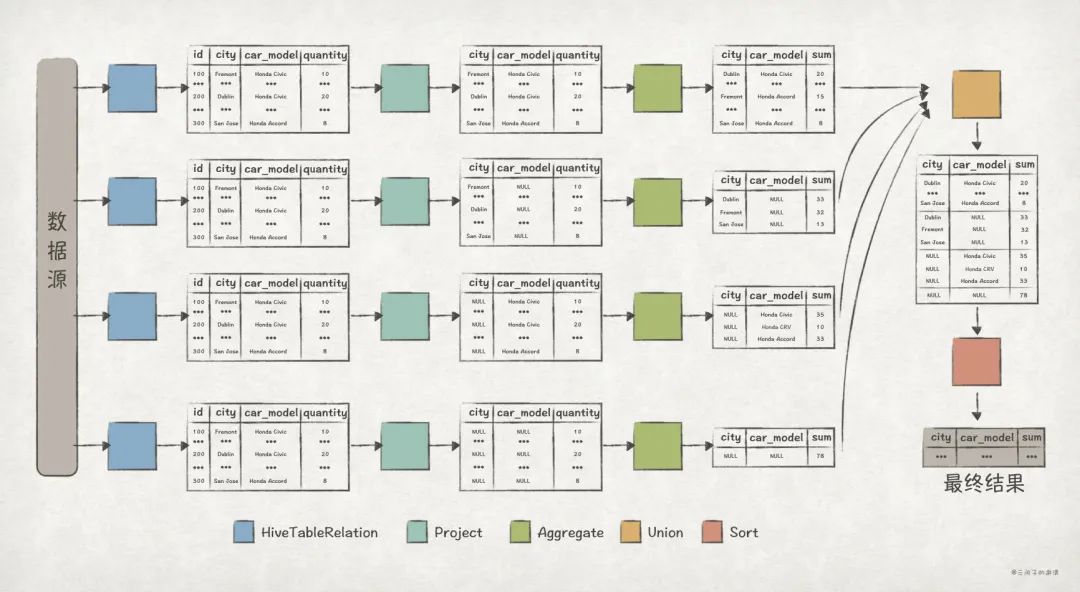
从上述的 Optimized Logical Plan 可以清晰地看出 Union All 版本的执行逻辑:
- 执行每个子查询语句,计算得出查询结果。其中,每个查询语句的逻辑是这样的:
- 在 HiveTableRelation 节点对
dealer表进行全表扫描。 - 在 Project 节点选出与查询语句结果相关的列,比如对于子查询语句
SELECT NULL as city, NULL as car_model, sum(quantity) AS sum FROM dealer,只需保留quantity列即可。 - 在 Aggregate 节点完成
quantity列对聚合运算。在上述的 Plan 中,Aggregate 后面紧跟的就是用来分组的列,比如Aggregate [city#902]就表示根据city列来进行分组。
- 在 HiveTableRelation 节点对
- 在 Union 节点完成对每个子查询结果的联合。
- 最后,在 Sort 节点完成对数据的排序,上述 Plan 中
Sort [city#93 ASC NULLS FIRST, car_model#94 ASC NULLS FIRST]就表示根据city和car_model列进行升序排序。
接下来,我们通过 explain extended 来查看 Grouping Sets 版本的 Optimized Logical Plan:
spark-sql> explain extended SELECT city, car_model, sum(quantity) AS sum FROM dealer GROUP BY GROUPING SETS ((city, car_model), (city), (car_model), ()) ORDER BY city, car_model;
== Parsed Logical Plan ==
...
== Analyzed Logical Plan ==
...
== Optimized Logical Plan ==
Sort [city#138 ASC NULLS FIRST, car_model#139 ASC NULLS FIRST], true
+- Aggregate [city#138, car_model#139, spark_grouping_id#137L], [city#138, car_model#139, sum(quantity#133) AS sum#124L]
   +- Expand [[quantity#133, city#131, car_model#132, 0], [quantity#133, city#131, null, 1], [quantity#133, null, car_model#132, 2], [quantity#133, null, null, 3]], [quantity#133, city#138, car_model#139, spark_grouping_id#137L]
      +- Project [quantity#133, city#131, car_model#132]
         +- HiveTableRelation [`default`.`dealer`, org.apache.hadoop.hive.serde2.lazy.LazySimpleSerDe, Data Cols: [id#130, city#131, car_model#132, quantity#133], Partition Cols: []]
== Physical Plan ==
...
从 Optimized Logical Plan 来看,Grouping Sets 版本要简洁很多!具体的执行逻辑是这样的:
- 在 HiveTableRelation 节点对
dealer表进行全表扫描。 - 在 Project 节点选出与查询语句结果相关的列。
- 接下来的 Expand 节点是关键,数据经过该节点后,多出了
spark_grouping_id列。从 Plan 中可以看出来,Expand 节点包含了Grouping Sets里的各个 grouping set 信息,比如[quantity#133, city#131, null, 1]对应的就是(city)这一 grouping set。而且,每个 grouping set 对应的spark_grouping_id列的值都是固定的,比如(city)对应的spark_grouping_id为1。 - 在 Aggregate 节点完成
quantity列对聚合运算,其中分组的规则为city, car_model, spark_grouping_id。注意,数据经过 Aggregate 节点后,spark_grouping_id列被删除了! - 最后,在 Sort 节点完成对数据的排序。

从 Optimized Logical Plan 来看,虽然 Union All 版本和 Grouping Sets 版本的效果一致,但它们的底层实现有着巨大的差别。
其中,Grouping Sets 版本的 Plan 中最关键的是 Expand 节点,目前,我们只知道数据经过它之后,多出了 spark_grouping_id 列。而且从最终结果来看,spark_grouping_id只是 Spark SQL 的内部实现细节,对用户并不体现。那么:
- Expand 的实现逻辑是怎样的,为什么能达到
Union All的效果? - Expand 节点的输出数据是怎样的 ?
spark_grouping_id列的作用是什么 ?
通过 Physical Plan,我们发现 Expand 节点对应的算子名称也是 Expand:
== Physical Plan ==
AdaptiveSparkPlan isFinalPlan=false
+- Sort [city#138 ASC NULLS FIRST, car_model#139 ASC NULLS FIRST], true, 0
   +- Exchange rangepartitioning(city#138 ASC NULLS FIRST, car_model#139 ASC NULLS FIRST, 200), ENSURE_REQUIREMENTS, [plan_id=422]
      +- HashAggregate(keys=[city#138, car_model#139, spark_grouping_id#137L], functions=[sum(quantity#133)], output=[city#138, car_model#139, sum#124L])
         +- Exchange hashpartitioning(city#138, car_model#139, spark_grouping_id#137L, 200), ENSURE_REQUIREMENTS, [plan_id=419]
            +- HashAggregate(keys=[city#138, car_model#139, spark_grouping_id#137L], functions=[partial_sum(quantity#133)], output=[city#138, car_model#139, spark_grouping_id#137L, sum#141L])
               +- Expand [[quantity#133, city#131, car_model#132, 0], [quantity#133, city#131, null, 1], [quantity#133, null, car_model#132, 2], [quantity#133, null, null, 3]], [quantity#133, city#138, car_model#139, spark_grouping_id#137L]
                  +- Scan hive default.dealer [quantity#133, city#131, car_model#132], HiveTableRelation [`default`.`dealer`, ..., Data Cols: [id#130, city#131, car_model#132, quantity#133], Partition Cols: []]
带着前面的几个问题,接下来我们深入 Spark SQL 的 Expand 算子源码寻找答案。
-
在Delphi中动态地使用SQL查询语句2009-05-10 0
-
SQL语句生成器2009-06-12 0
-
关于labview中的SQL语句写法2013-01-05 0
-
C语言深度剖析2019-03-19 0
-
SQL语句的两种嵌套方式2019-05-23 0
-
区分SQL语句与主语言语句2021-10-28 0
-
为什么要动态sql语句?2021-12-20 0
-
嵌入式SQL语句与主语言之间的通信2021-12-22 0
-
数据库SQL语句电子教程2011-07-14 833
-
如何使用navicat或PHPMySQLAdmin导入SQL语句2018-04-10 654
-
如何使用SQL修复语句程序说明2019-10-31 554
-
嵌入式SQL语句2021-10-21 438
-
深度剖析SQL中的Grouping Sets语句22023-05-10 382
-
sql查询语句大全及实例2023-11-17 678
-
oracle执行sql查询语句的步骤是什么2023-12-06 432
全部0条评论

快来发表一下你的评论吧 !
