锁相环仿真_MATLAB仿真程序代码_二阶锁相环仿真过程

　　本蚊介绍了仿真的环境以及二阶锁相环的仿真过程，并对其仿真结果进行了分析。在前三章的理论基础上，通过使用MATLAB7.0进行了仿真。

　　验结果表明：用MATLAB进行的二阶锁相环仿真达到了最初的设想，锁相环的失锁、跟踪、捕获、锁定各个阶段均有体现。达到了最初仿真的要求。

（典型仿真案例）图

　　仿真使用软件MATLAB7.0

　　仿真使用的软件是MATLAB7.0。由于MATLAB仿真软件适合多学科、多种工作平台且功能强大、界面友好、方便快捷、语言自然并且开放性强的大型优秀应用软件，已经也已成为国内外高等院校高等数学、数值分析、数字信号处理、自动控制理论以及工程应用等课程的基本教学工具。使用Matlab对锁相环仿真的实现是方便快捷的。

　　仿真采用二阶锁相环

　　仿真所采用的是二阶锁相环。这是由于我们实际应用中的绝大多数PLL，或者是二阶的，或者是通过忽略高阶效应（至少在初步设计时）而被设计成近似的二阶环路。鉴于二阶锁相环在实际应用的意义，所以在仿真采用了二阶锁相环。

　　MATLAB仿真程序代码

　　% File： c6_nltvde.m

　　w2b=0; w2c=0; % initialize integrators

　　yd=0; y=0; % initialize differential equation

　　tfinal = 50; % simulation time

　　fs = 100; % sampling frequency

　　delt = 1/fs; % sampling period

　　npts = 1+fs*tfinal; % number of samples simulated

　　ydv = zeros（1，npts）; % vector of dy/dt samples

　　yv = zeros（1，npts）; % vector of y（t） samples

　　%

　　% beginning of simulation loop for i=1:npts t = （i-1）*delt;

　　% time

　　if t《20

　　ydd = 4*exp（-t/2）-3*yd*abs（y）-9*y; % de for t《20

　　else

　　ydd = 4*exp（-t/2）-3*yd-9*y;

　　% de for t》=20 end

　　w1b=ydd+w2b; % first integrator - step 1 w2b=ydd+w1b;

　　% first integrator - step 2

　　yd=w1b/（2*fs）; % first integrator output w1c=yd+w2c; % second integrator - step 1 w2c=yd+w1c;

　　% second integrator - step 2

　　y=w1c/（2*fs）; % second integrator output ydv（1，i） = yd; % build dy/dt vector yv（1，i） = y; % build y（t） vector end

　　% end of simulation loop

　　plot（yv，ydv） % plot phase plane xlabel（‘y（t）’） % label x axis ylabel（‘dy/dt’）

　　% label y zxis

　　% End of script file. % File： pllpost.m

　　%

　　kk = 0; while kk == 0 k = menu（‘Phase Lock Loop Postprocessor’，。。。

　　‘Input Frequency and VCO Frequency’，。。。

　　‘Input Phase and VCO Phase’，。。。

　　‘Frequency Error’，‘Phase Error’，‘Phase Plane Plot’，。。。

　　‘Phase Plane and Time Domain Plots’，‘Exit Program’）;

　　if k == 1

　　plot（t，fin，‘k’，t，fvco，‘k’）

　　title（‘Input Frequency and VCO Freqeuncy’）

　　xlabel（‘Time - Seconds’）;ylabel（‘Frequency - Hertz’）;pause

　　elseif k ==2

　　pvco=phin-phierror;plot（t，phin，t，pvco）

　　title（‘Input Phase and VCO Phase’）

　　xlabel（‘Time - Seconds’）;ylabel（‘Phase - Radians’）;pause

　　elseif k == 3 plot

　　（t，freqerror）;title（‘Frequency Error’）

　　xlabel（‘Time - Seconds’）;ylabel（‘Frequency Error - Hertz’）;pause

　　elseif k == 4

　　plot（t，phierror）;title（‘Phase Error’）

　　xlabel（‘Time - Seconds’）;ylabel（‘Phase Error - Radians’）;pause

　　elseif k == 5

　　ppplot

　　elseif k == 6

　　subplot（211）;phierrn = phierror/pi;

　　plot（phierrn，freqerror，‘k’）;grid;

　　title（‘Phase Plane Plot’）;xlabel（‘Phase Error /Pi’）;

　　ylabel（‘Frequency Error - Hertz’）;subplot（212）

　　plot（t，fin，‘k’，t，fvco，‘k’）;grid

　　title（‘Input Frequency and VCO Freqeuncy’）

　　xlabel（‘Time - Seconds’）;ylabel（‘Frequency - Hertz’）;subplot（111）

　　elseif k == 7

　　kk = 1;

　　end

　　end % End of script file.

　　% File： pllpre.m

　　%

　　clear all % be safe

　　disp（‘ ’） % insert blank line

　　fdel = input（‘Enter the size of the frequency step in Hertz 》 ’）;

　　fn = input（‘Enter the loop natural frequency in Hertz 》 ’）;

　　lambda = input（‘Enter lambda， the relative pole offset 》 ’）;

　　disp（‘ ’）

　　disp（‘Accept default values：’）

　　disp（‘ zeta = 1/sqrt（2） = 0.707，’）

　　disp（‘ fs = 200*fn， and’）

　　disp（‘ tstop = 1’） dtype = input（‘Enter y for yes or n for no 》 ’，‘s’）;

　　if dtype == ‘y’

　　zeta = 1/sqrt（2）;

　　fs = 200*fn;

　　tstop = 1;

　　else

　　zeta = input（‘Enter zeta， the loop damping factor 》 ’）;

　　fs = input（‘Enter the sampling frequency in Hertz 》 ’）;

　　tstop = input（‘Enter tstop， the simulation runtime 》 ’）;

　　end %

　　npts = fs*tstop+1; % number of simulation points

　　t = （0：（npts-1））/fs; % default time vector

　　nsettle = fix（npts/10）; % set nsettle time as 0.1*npts

　　tsettle = nsettle/fs; % set tsettle

　　% The next two lines establish the loop input frequency and phase

　　% deviations.

　　fin = ［zeros（1，nsettle），fdel*ones（1，npts-nsettle）］;

　　phin = ［zeros（1，nsettle），2*pi*fdel*t（1：（npts-nsettle））］;

　　disp（‘ ’） % insertblank line

　　% end of script file pllpre.m

　　% File： pll2sin.m

　　w2b=0; w2c=0; s5=0; phivco=0; %initialize

　　twopi=2*pi; % define 2*pi

　　twofs=2*fs; % define 2*fs

　　G=2*pi*fn*（zeta+sqrt（zeta*zeta-lambda））; % set loop gain

　　a=2*pi*fn/（zeta+sqrt（zeta*zeta-lambda））; % set filter parameter

　　a1=a*（1-lambda）; a2 = a*lambda; % define constants

　　phierror = zeros（1，npts）; % initialize vector

　　fvco=zeros（1，npts）; % initialize vector

　　% beginning of simulation loop

　　for i=1:npts

　　s1=phin（i） - phivco; % phase error

　　s2=sin（s1）; % sinusoidal phase detector

　　s3=G*s2;

　　s4=a1*s3;

　　s4a=s4-a2*s5; % loop filter integrator input

　　w1b=s4a+w2b; % filter integrator （step 1）

　　w2b=s4a+w1b; % filter integrator （step 2）

　　s5=w1b/twofs; % generate fiter output

　　s6=s3+s5; % VCO integrator input

　　w1c=s6+w2c; % VCO integrator （step 1）

　　w2c=s6+w1c; % VCO integrator （step 2）

　　phivco=w1c/twofs; % generate VCO output

　　phierror（i）=s1; % build phase error vector

　　fvco（i）=s6/twopi; % build VCO input vector

　　end

　　% end of simulation loop

　　freqerror=fin-fvco; % build frequency error vector

　　% End of script file.

　　function ［］ = pplane（x，y，nsettle）

　　% Plots the phase plane with phase in the range （-pi，pi）

　　ln = length（x）;

　　maxfreq = max（y）;

　　minfreq = min（y）;

　　close % Old figure discarded

　　axis（［-1 1 1.1*minfreq 1.1*maxfreq］）; % Establish scale

　　hold on % Collect info for new fig

　　j = nsettle; while j 《 ln

　　i = 1;

　　while x（j） 《 pi & j 《 ln

　　a（i） = x（j）/pi;

　　b（i） = y（j）;

　　j = j+1;

　　i = i+1;

　　end

　　plot（a，b，‘k’）

　　a = ［］;

　　b = ［］;

　　x = x - 2*pi;

　　end hold off title（‘Phase-Plane Plot’）

　　xlabel（‘Phase Error / Pi’）

　　ylabel（‘Frequency Error in Hertz’）

　　grid % End of script file.

　　% File： ppplot.m

　　% ppplot.m is the script file for plotting phase plane plots. If the

　　% phase plane is constrained to （-pi，pi） ppplot.m calls pplane.m.

　　kz = 0;

　　仿真过程及结果

　　

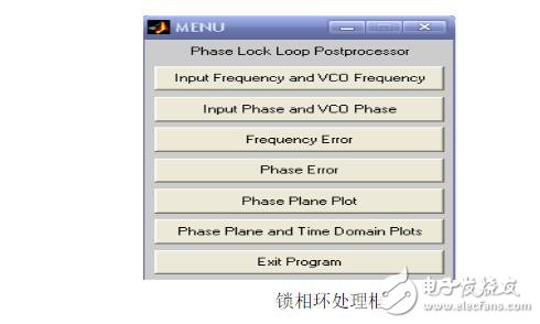
　　上图是利用MATLAB提供的函数将计算结果图形化功能建立的。在运行程序后，就会出现上面的对话框，点击点击其中的任何一项就会出现相应的仿真图形。上图中包含了输入频率和VCO频率，输入相位和VCO相位，频率误差，相位误差，相位空间波特图，相位空间和时域，退出程序等选项。运行程序后出现如下指令：

　　Accept the tentative values： the first loop frequency is 5 第一循环频率

　　Enter y for yes or n for no 》 y

　　Enter the loop gain 》40 输入环路增益为

　　40 Enter the sampling frequency in Hertz 》 1200 输入采样频率

　　Enter tstop， the simulation runtime 》 5 仿真时间为5秒

　　设置好参数后运行程序，由上我们可知环路增益为40，仿真时间为5s，采样频率为1200Hz。接着点击上图锁相环处理框中的菜单，就能得到如下仿真图像。其中我们主要观察输入相位和VCO相位。

　　

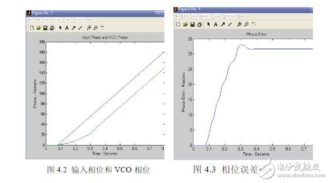
　　图4.2中蓝线为输入相位，绿线代表VCO相位，从图中可以看见随着时间的变化输入信号相位为线性，而VCO相位则是经历了一段曲线后斜率与输入信号相位斜率相同，输出相位跟随输入相位，达到稳定。图4.3中VCO的相位也是先经历了一段时间的曲线后变为一条直线达到稳定。根据锁相环的基本原理我们可知锁相环是个反馈网络，它是由输出信号（VCO产生）与参考频率在频率和相位上保持同步或者保持常数。由此我们可以看出锁相环工作后，在最初的一段时间中锁相环开始工作，输入信号经过鉴相器，环路虑波器后，将输出相位反馈给VCO压控振荡器，使压控振荡器与输入频率逐步实现同步，保持一个常数，实现锁定。其中经历了锁相环的失锁、跟踪、捕获、锁定，从而达到最后达到稳定状态。从开始到达到稳定的这段时间则为做捕获时间。

　　

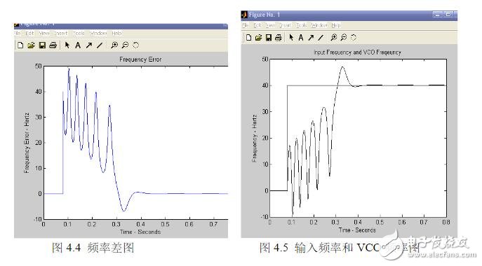
　　图4..4与图4.5也显示了锁相环工作后从失锁、跟踪、捕获、锁定的过程，过程。从不停的摆动到最后的直线状态，这个过程称为锁定过程。其中我们可以发现在捕捉过程中随着捕捉次数的增加，捕捉过程也变得较慢，这说明此时的的锁相环工作平率处在稳定工作的动态界限内，工作正常。