NAC的工作原理，以及它如何处理加法和减法等操作

Tensorflowers 2018-10-10 6537

描述

DeepMind 最近发布了一篇新的论文---《神经算术逻辑单元（NALU）》（https://arxiv.org/abs/1808.00508），这是一篇很有趣的论文，它解决了深度学习中的一个重要问题，即教导神经网络计算。令人惊讶的是，尽管神经网络已经能够在许多任务，如肺癌分类中获得卓绝表现，却往往在一些简单任务，像计算数字上苦苦挣扎。

在一个展示网络如何努力从新数据中插入特征的实验中，我们的研究发现，他们能够用 -5 到 5 之间的数字将训练数据分类，准确度近乎完美，但对于训练数据之外的数字，网络几乎无法归纳概括。

论文提供了一个解决方案，分成两个部分。以下我将简单介绍一下 NAC 的工作原理，以及它如何处理加法和减法等操作。之后，我会介绍 NALU，它可以处理更复杂的操作，如乘法和除法。我提供了可以尝试演示这些代码的代码，您可以阅读上述的论文了解更多详情。

深度学习

第一神经网络（NAC）

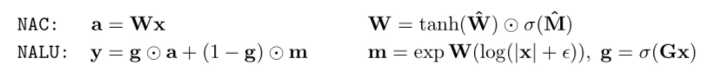
神经累加器（简称 NAC）是其输入的一种线性变换。什么意思呢？它是一个转换矩阵，是 tanh（W_hat）和 sigmoid（M_hat）的元素乘积。最后，转换矩阵 W 乘以输入（x）。

Python 中的 NAC

1 import tensorflow as tf

3 # NAC

4 W_hat = tf.Variable(tf.truncated_normal(shape, stddev=0.02))

5 M_hat = tf.Variable(tf.truncated_normal(shape, stddev=0.02))

7 W = tf.tanh(W_hat) * tf.sigmoid(M_hat)

8 # Forward propogation

9 a = tf.matmul(in_dim, W)

NAC

第二神经网络 (NALU)

神经算术逻辑单元，或者我们简称之为 NALU，是由两个 NAC 单元组成。第一个 NAC g 等于 sigmoid（Gx）。第二个 NAC 在一个等于 exp 的日志空间 m 中运行 (W(log(|x| + epsilon)))

Python 中的 NALU

1 import tensorflow as tf

3 # NALU

4 G = tf.Variable(tf.truncated_normal(shape, stddev=0.02))

6 m = tf.exp(tf.matmul(tf.log(tf.abs(in_dim) + epsilon), W))

8 g = tf.sigmoid(tf.matmul(in_dim, G))

10 y = g * a + (1 - g) * m

NALU

通过学习添加来测试 NAC

现在让我们进行测试，首先将 NAC 转换为函数。

1 # Neural Accumulator

2 def NAC(in_dim, out_dim):

4 in_features = in_dim.shape[1]

6 # define W_hat and M_hat

7 W_hat = tf.get_variable(name = 'W_hat', initializer=tf.initializers.random_uniform(minval=-2, maxval=2),shape=[in_features, out_dim], trainable=True)

8 M_hat = tf.get_variable(name = 'M_hat', initializer=tf.initializers.random_uniform(minval=-2, maxval=2), shape=[in_features, out_dim], trainable=True)

10 W = tf.nn.tanh(W_hat) * tf.nn.sigmoid(M_hat)

12 a = tf.matmul(in_dim, W)

14 return a, W

NAC function in Python

Python 中的 NAC 功能

接下来，让我们创建一些玩具数据，用于训练和测试数据。 NumPy 有一个名为 numpy.arrange 的优秀 API，我们将利用它来创建数据集。

1 # Generate a series of input number X1 and X2 for training

2 x1 = np.arange(0,10000,5, dtype=np.float32)

3 x2 = np.arange(5,10005,5, dtype=np.float32)

6 y_train = x1 + x2

8 x_train = np.column_stack((x1,x2))

10 print(x_train.shape)

11 print(y_train.shape)

13 # Generate a series of input number X1 and X2 for testing

14 x1 = np.arange(1000,2000,8, dtype=np.float32)

15 x2 = np.arange(1000,1500,4, dtype= np.float32)

17 x_test = np.column_stack((x1,x2))

18 y_test = x1 + x2

20 print()

21 print(x_test.shape)

22 print(y_test.shape)

添加玩具数据

现在，我们可以定义样板代码来训练模型。我们首先定义占位符 X 和 Y，用以在运行时提供数据。接下来我们定义的是 NAC 网络（y_pred，W = NAC（in_dim = X，out_dim = 1））。对于损失，我们使用 tf.reduce_sum()。我们将有两个超参数，alpha，即学习率和我们想要训练网络的时期数。在运行训练循环之前，我们需要定义一个优化器，这样我们就可以使用 tf.train.AdamOptimizer() 来减少损失。

1 # Define the placeholder to feed the value at run time

2 X = tf.placeholder(dtype=tf.float32, shape =[None , 2]) # Number of samples x Number of features (number of inputs to be added)

3 Y = tf.placeholder(dtype=tf.float32, shape=[None,])

5 # define the network

6 # Here the network contains only one NAC cell (for testing)

7 y_pred, W = NAC(in_dim=X, out_dim=1)

8 y_pred = tf.squeeze(y_pred) # Remove extra dimensions if any

10 # Mean Square Error (MSE)

11 loss = tf.reduce_mean( (y_pred - Y) **2)

14 # training parameters

15 alpha = 0.05 # learning rate

16 epochs = 22000

18 optimize = tf.train.AdamOptimizer(learning_rate=alpha).minimize(loss)

20 with tf.Session() as sess:

22 #init = tf.global_variables_initializer()

23 cost_history = []

25 sess.run(tf.global_variables_initializer())

27 # pre training evaluate

28 print("Pre training MSE: ", sess.run (loss, feed_dict={X: x_test, Y:y_test}))

29 print()

30 for i in range(epochs):

31 _, cost = sess.run([optimize, loss ], feed_dict={X:x_train, Y: y_train})

32 print("epoch: {}, MSE: {}".format( i,cost) )

33 cost_history.append(cost)

35 # plot the MSE over each iteration

36 plt.plot(np.arange(epochs),np.log(cost_history)) # Plot MSE on log scale

37 plt.xlabel("Epoch")

38 plt.ylabel("MSE")

39 plt.show()

41 print()

42 print(W.eval())

43 print()

44 # post training loss

45 print("Post training MSE: ", sess.run(loss, feed_dict={X: x_test, Y: y_test}))

47 print("Actual sum: ", y_test[0:10])

48 print()

49 print("Predicted sum: ", sess.run(y_pred[0:10], feed_dict={X: x_test, Y: y_test}))

训练之后，成本图的样子：

深度学习

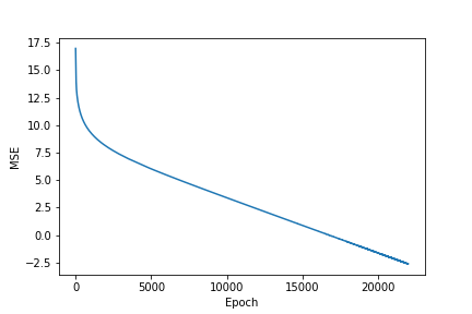
NAC 训练之后的成本

Actual sum: [2000. 2012. 2024. 2036. 2048. 2060. 2072. 2084. 2096. 2108.]Predicted sum: [1999.9021 2011.9015 2023.9009 2035.9004 2047.8997 2059.8992 2071.8984 2083.898 2095.8975 2107.8967]

虽然 NAC 可以处理诸如加法和减法之类的操作，但是它无法处理乘法和除法。于是，就有了 NALU 的用武之地。它能够处理更复杂的操作，例如乘法和除法。

通过学习乘法来测试 NALU

为此，我们将添加片段以使 NAC 成为 NALU。

深度学习

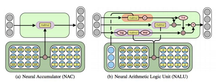
神经累加器（NAC）是其输入的线性变换。神经算术逻辑单元（NALU）使用两个带有绑定的权重的 NACs 来启用加法或者减法（较小的紫色单元）和乘法/除法（较大的紫色单元），由一个门（橙色单元）来控制。

1 # The Neural Arithmetic Logic Unit

2 def NALU(in_dim, out_dim):

4 shape = (int(in_dim.shape[-1]), out_dim)

5 epsilon = 1e-7

7 # NAC

8 W_hat = tf.Variable(tf.truncated_normal(shape, stddev=0.02))

9 M_hat = tf.Variable(tf.truncated_normal(shape, stddev=0.02))

10 G = tf.Variable(tf.truncated_normal(shape, stddev=0.02))

12 W = tf.tanh(W_hat) * tf.sigmoid(M_hat)

13 # Forward propogation

14 a = tf.matmul(in_dim, W)

16 # NALU

17 m = tf.exp(tf.matmul(tf.log(tf.abs(in_dim) + epsilon), W))

18 g = tf.sigmoid(tf.matmul(in_dim, G))

19 y = g * a + (1 - g) * m

21 return y

Python 中的 NALU 函数

现在，再次创建一些玩具数据，这次我们将进行两行更改。

1 # Test the Network by learning the multiplication

3 # Generate a series of input number X1 and X2 for training

4 x1 = np.arange(0,10000,5, dtype=np.float32)

5 x2 = np.arange(5,10005,5, dtype=np.float32)

8 y_train = x1 * x2

10 x_train = np.column_stack((x1,x2))

12 print(x_train.shape)

13 print(y_train.shape)

15 # Generate a series of input number X1 and X2 for testing

16 x1 = np.arange(1000,2000,8, dtype=np.float32)

17 x2 = np.arange(1000,1500,4, dtype= np.float32)

19 x_test = np.column_stack((x1,x2))

20 y_test = x1 * x2

22 print()

23 print(x_test.shape)

24 print(y_test.shape)

用于乘法的玩具数据

第 8 行和第 20 行是进行更改的地方，将加法运算符切换为乘法。

现在我们可以训练的是 NALU 网络。我们唯一需要更改的地方是定义 NAC 网络改成 NALU（y_pred = NALU（in_dim = X，out_dim = 1））。

1 # Define the placeholder to feed the value at run time

2 X = tf.placeholder(dtype=tf.float32, shape =[None , 2]) # Number of samples x Number of features (number of inputs to be added)

3 Y = tf.placeholder(dtype=tf.float32, shape=[None,])

5 # Define the network

6 # Here the network contains only one NAC cell (for testing)

7 y_pred = NALU(in_dim=X, out_dim=1)

8 y_pred = tf.squeeze(y_pred) # Remove extra dimensions if any

10 # Mean Square Error (MSE)

11 loss = tf.reduce_mean( (y_pred - Y) **2)

14 # training parameters

15 alpha = 0.05 # learning rate

16 epochs = 22000

18 optimize = tf.train.AdamOptimizer(learning_rate=alpha).minimize(loss)

20 with tf.Session() as sess:

22 #init = tf.global_variables_initializer()

23 cost_history = []

25 sess.run(tf.global_variables_initializer())

27 # pre training evaluate

28 print("Pre training MSE: ", sess.run (loss, feed_dict={X: x_test, Y: y_test}))

29 print()

30 for i in range(epochs):

31 _, cost = sess.run([optimize, loss ], feed_dict={X: x_train, Y: y_train})

32 print("epoch: {}, MSE: {}".format( i,cost) )

33 cost_history.append(cost)

35 # Plot the loss over each iteration

36 plt.plot(np.arange(epochs),np.log(cost_history)) # Plot MSE on log scale

37 plt.xlabel("Epoch")

38 plt.ylabel("MSE")

39 plt.show()

42 # post training loss

43 print("Post training MSE: ", sess.run(loss, feed_dict={X: x_test, Y: y_test}))

45 print("Actual product: ", y_test[0:10])

46 print()

47 print("Predicted product: ", sess.run(y_pred[0:10], feed_dict={X: x_test, Y: y_test}))

NALU 训练后的成本

Actual product: [1000000. 1012032. 1024128. 1036288. 1048512. 1060800. 1073152. 1085568. 1098048. 1110592.]Predicted product: [1000000.2 1012032. 1024127.56 1036288.6 1048512.06 1060800.8 1073151.6 1085567.6 1098047.6 1110592.8 ]

在 TensorFlow 中全面实现

打开APP阅读更多精彩内容