

理解积分非线性误差-Understanding Integr
AD技术
11人已加入
描述
Abstract: To understand the effects of integral non-linearity errors, the most straightforward approach is to analyze a simple sine wave and apply well-known trigonometric identities to a non-ideal, analog-to-digital output transfer function, which contains an INL error.
With an ideal system, a single-tone sine wave with amplitude A and frequency fo,
X(t) = Asin(2π fot)
Sampling with an ADC with a period of T results in a discrete signal:
X[n]=Asin(2π fonT),
where X[n] is the discrete-time signal obtained from the uniform sampling of X(t) every T seconds. The reciprocal 1/T = F is called the sampling rate or sampling frequency.
A particularly important class of systems consists of those that are linear and time invariant, or "LTI." These two properties in combination lead to especially convenient representations for such systems. Most important, the relationship between the input to a LTI system X[n] and the output Y[n] can be given by a convolution sum. Convolution is fundamental to the analysis and description of LTI systems. In this example, we will only be analyzing the linearity of a system.
A linear system is one that satisfies the superposition principle. Simply stated, the principle of superposition requires that the response of the system to a weighted sum of signals be equal to the corresponding weighted sum of the responses (outputs) of the system to each individual input signals. The superposition property greatly simplifies the analysis of linear systems. Because of the decomposition property, you can evaluate separately the different components of the output.
Comparing an ideal ADC transfer curve to a transfer curve with an INL error, it is easy to demonstrate how a system with INL error yields a non-linear output. The output Y3[n] is not equal to the sum of output Y1[n] +Y2[n] when its input is X3[n] = X1[n] + X2[n]. More precisely, F(X1 + X2) ≠ F(X1) + F(X2). As a result, the non-linearity error produces additional, unwanted, internally generated sinusoids which can increase the design cost and the filter complexity. (Electrical engineers recognize this effect of internally generated sinusoids as intermodulation distortion.)
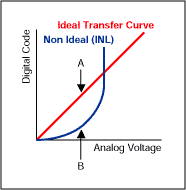
Figure 1. The distance between the tip of arrow A and the tip of arrow B, is a measurement of the INL error.
In the above figure, the ideal transfer function is draw as a straight linear line. In this example, the non ideal transfer curve, which includes INL error, is drawn just as a second order function Y[n] = k[X[n]]^2. In reality, the non ideal transfer function may also contain second order, third order, fourth order, etc., components Y[n] = kX1[n] + k2X[n]^2 + k3X[n]^3 + k4X[n]^4 + ...
For the following analysis, only the second order component is considered.
X1[n] = sin(2π × fo × nT) fo = 1Hz (separated out fo for clarity), amplitude A=1, no phase
Y1[n] = kX1[n]X1[n] set constant k = 1 for simplicity in this example
Y1[n] = sin(2π × 1 × nT)sin(2π × 1 × nT)
Note: Recall from trigonometry identities, Sin(A)Sin(B) = Cos(A-B)/2 - Cos(A+B)/2
Y1[n] = cos(2π × 1 × nT - 2π × 1 × nT)/2 - cos(2π × 1 × nT + 2π × 1 × nT)/2
Y1[n] = cos(0)/2 - cos(4π × 1 × nT)/2
Y1[n] = 1/2 - cos(2π × 2 × nT)/2 (cosine wave with fo = 2Hz and peak amplitude of -0.5)
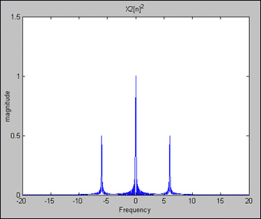
Figure 2. Y2[n] = X2[n]2 = 1/2 - cos(2π × 6 × nT)/2.
X2[n] = sin(2π × fo × nT) with fo = 3Hz with an amplitude A=1
Y2[n] = sin(2π × 3 × nT)sin(2π × 3 × nT)
Y2[n] = cos(2π × 3 × nT - 2π × 3 × nT)/2 - cos(2π × 3 × nT + 2π × 3 × nT)/2
Y2[n] = cos(0)/2 - cos(4π × 3 × nT)/2
Y2[n] = 1/2 - cos(2π × 6 × nT)/2 (cosine wave with fo = 6Hz and peak amplitude of -0.5)
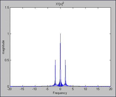
Figure 3. Y1[n] = X1[n]2 = 1/2 - cos(2π × 2 × nT)/2.
We can now apply X3[n] = X1[n] + X2[n] , with Y3[n] = [X[3]]^2
Y3[n] = [ X1[n] + X2[n] ]^2
Y3[n] = X1[n]X1[n] + 2 X1[n]X2[n] + X2[n]X2[n]
As previously noted:
X1[n]X1[n] results in a constant value of 1/2 and a cosine wave of 2Hz, amplitude -0.5
X2[n]X2[n] results in a constant value of 1/2 and a cosine wave of 6Hz, amplitude -0.5
Therefore,
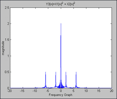
Figure 4. Y3[n] = X1[n]^2 = 1 - cos(2π × 2 × nT)/2 - cos(2π × 6 × nT)/2.
However,
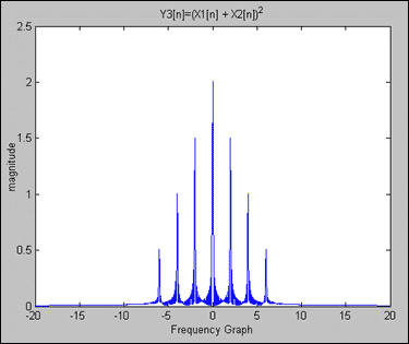
Figure 5. Y3[n] = X1[n] + X2[n])^2 = 1 - cos(2π × 2 × nT)/2 - cos(2π × 6 × nT)/2 + cos(2π × 4 × nT).
As a result of the integral non-linearity error, we have added two additional cosine waves of 2Hz and 4Hz. The superposition principle is not satisfied, therefore the system is non-linear and is not a Linear Time Invariant system. As noted above, filtering needs to be applied to suppress the additional unwanted frequencies (or side lobes), adding design complexity and cost.
% Maxim Integrated Products
% Magnitude Verses Frequency Plots - Non-Linearity Error
n = 0:1023;
w0 = 0.02*pi; % w0 = 2*pi*1*0.01 , frequency = 1Hz, Sample period = .01s
w1 = 0.06*pi; % w1 = 2*pi*3*0.01 , frequency = 3Hz, Sample period = .01s
N = 2048;
w = (-N/2:(N-1)/2)*2*pi/N;
x1=cos(w0*n); % X1[n] = cos(2*pi*1*n*0.01) freq = 1Hz , Sample period = .01s
x2=cos(w1*n); % X2[n] = cos(2*pi*3*n*0.01) freq = 3Hz , Sample period = .01s
x3=x1+x2;
y1=x1.*x1; % Y1[n] = [X1[n]]^2
y2=x2.*x2; % Y2[n] = [X2[n]]^2
y3=y1+y2;
y4=x3.*x3;
L = 1024;
Z0=[y1(1:L) zeros(1, 2048 - L)];
Z1=[y2(1:L) zeros(1, 2048 - L)];
Z2=[y3(1:L) zeros(1, 2048 - L)];
Z3=[y4(1:L) zeros(1, 2048 - L)];
%Perform FFT on signals
Z5=fft(Z0, N);
fftshift(Z5);
Z6=fft(Z1, N);
fftshift(Z6);
Z7=fft(Z2, N);
fftshift(Z7);
Z8=fft(Z3, N);
fftshift(Z8);
%Plot signals
subplot(2,2,1);plot(w/(.02*pi),abs(fftshift(Z5)/512)), xlabel(''), ylabel('magnitude');
title('X1[n]^2');
subplot(2,2,2);plot(w/(.02*pi),abs(fftshift(Z6)/512)), xlabel(''), ylabel('magnitude');
title('X2[n]^2');
subplot(2,2,3);plot(w/(.02*pi),abs(fftshift(Z7)/512)), xlabel('Frequency Graph'), ylabel('magnitude');
title('Y3[n]=X1[n]^2 + X2[n]^2');
subplot(2,2,4);plot(w/(.02*pi),abs(fftshift(Z8)/512)), xlabel('Frequency Graph'), ylabel('magnitude');
title('Y3[n]=(X1[n] + X2[n])^2');
打开APP阅读更多精彩内容
With an ideal system, a single-tone sine wave with amplitude A and frequency fo,
X(t) = Asin(2π fot)
Sampling with an ADC with a period of T results in a discrete signal:
X[n]=Asin(2π fonT),
where X[n] is the discrete-time signal obtained from the uniform sampling of X(t) every T seconds. The reciprocal 1/T = F is called the sampling rate or sampling frequency.
A particularly important class of systems consists of those that are linear and time invariant, or "LTI." These two properties in combination lead to especially convenient representations for such systems. Most important, the relationship between the input to a LTI system X[n] and the output Y[n] can be given by a convolution sum. Convolution is fundamental to the analysis and description of LTI systems. In this example, we will only be analyzing the linearity of a system.
A linear system is one that satisfies the superposition principle. Simply stated, the principle of superposition requires that the response of the system to a weighted sum of signals be equal to the corresponding weighted sum of the responses (outputs) of the system to each individual input signals. The superposition property greatly simplifies the analysis of linear systems. Because of the decomposition property, you can evaluate separately the different components of the output.
Comparing an ideal ADC transfer curve to a transfer curve with an INL error, it is easy to demonstrate how a system with INL error yields a non-linear output. The output Y3[n] is not equal to the sum of output Y1[n] +Y2[n] when its input is X3[n] = X1[n] + X2[n]. More precisely, F(X1 + X2) ≠ F(X1) + F(X2). As a result, the non-linearity error produces additional, unwanted, internally generated sinusoids which can increase the design cost and the filter complexity. (Electrical engineers recognize this effect of internally generated sinusoids as intermodulation distortion.)

Figure 1. The distance between the tip of arrow A and the tip of arrow B, is a measurement of the INL error.
In the above figure, the ideal transfer function is draw as a straight linear line. In this example, the non ideal transfer curve, which includes INL error, is drawn just as a second order function Y[n] = k[X[n]]^2. In reality, the non ideal transfer function may also contain second order, third order, fourth order, etc., components Y[n] = kX1[n] + k2X[n]^2 + k3X[n]^3 + k4X[n]^4 + ...
For the following analysis, only the second order component is considered.
X1[n] = sin(2π × fo × nT) fo = 1Hz (separated out fo for clarity), amplitude A=1, no phase
Y1[n] = kX1[n]X1[n] set constant k = 1 for simplicity in this example
Y1[n] = sin(2π × 1 × nT)sin(2π × 1 × nT)
Note: Recall from trigonometry identities, Sin(A)Sin(B) = Cos(A-B)/2 - Cos(A+B)/2
Y1[n] = cos(2π × 1 × nT - 2π × 1 × nT)/2 - cos(2π × 1 × nT + 2π × 1 × nT)/2
Y1[n] = cos(0)/2 - cos(4π × 1 × nT)/2
Y1[n] = 1/2 - cos(2π × 2 × nT)/2 (cosine wave with fo = 2Hz and peak amplitude of -0.5)

Figure 2. Y2[n] = X2[n]2 = 1/2 - cos(2π × 6 × nT)/2.
X2[n] = sin(2π × fo × nT) with fo = 3Hz with an amplitude A=1
Y2[n] = sin(2π × 3 × nT)sin(2π × 3 × nT)
Y2[n] = cos(2π × 3 × nT - 2π × 3 × nT)/2 - cos(2π × 3 × nT + 2π × 3 × nT)/2
Y2[n] = cos(0)/2 - cos(4π × 3 × nT)/2
Y2[n] = 1/2 - cos(2π × 6 × nT)/2 (cosine wave with fo = 6Hz and peak amplitude of -0.5)

Figure 3. Y1[n] = X1[n]2 = 1/2 - cos(2π × 2 × nT)/2.
We can now apply X3[n] = X1[n] + X2[n] , with Y3[n] = [X[3]]^2
Y3[n] = [ X1[n] + X2[n] ]^2
Y3[n] = X1[n]X1[n] + 2 X1[n]X2[n] + X2[n]X2[n]
As previously noted:
X1[n]X1[n] results in a constant value of 1/2 and a cosine wave of 2Hz, amplitude -0.5
X2[n]X2[n] results in a constant value of 1/2 and a cosine wave of 6Hz, amplitude -0.5
| For 2X1[n]X2[n] | = 2sin(2π × 1 × nT)sin(2π × 3 × nT) |
| = cos(2π × 1 × nT - 2π × 3 × nT) - cos(2π × 1 × nT + 2π × 3 × nT) | |
| = cos(-4π × nT) - cos(8π × nT) | |
| = cos(-2π × 2 × nT) - cos(2π × 4 × nT) | |
| = cos(2π × 2 × nT) - cos(2π × 4 × nT) (cosine waves of 2Hz and 4Hz) |
Therefore,
| For Y3[n] | = X1[n]^2 + X2[n]^2 |
| = Y1[n] + Y2[n] | |
| = 1 - cos(2π × 2 × nT)/2 - cos(2π × 6 × nT)/2 |

Figure 4. Y3[n] = X1[n]^2 = 1 - cos(2π × 2 × nT)/2 - cos(2π × 6 × nT)/2.
However,
| For Y3[n] | = ( X1[n] + X2[n] )^2 |
| = 1 - cos(2π × 2 × nT)/2 - cos(2π × 6 × nT)/2 + cos(2π × 2 × nT) - cos(2π × 4 × nT) |

Figure 5. Y3[n] = X1[n] + X2[n])^2 = 1 - cos(2π × 2 × nT)/2 - cos(2π × 6 × nT)/2 + cos(2π × 4 × nT).
As a result of the integral non-linearity error, we have added two additional cosine waves of 2Hz and 4Hz. The superposition principle is not satisfied, therefore the system is non-linear and is not a Linear Time Invariant system. As noted above, filtering needs to be applied to suppress the additional unwanted frequencies (or side lobes), adding design complexity and cost.
Listing 1: Matlab Code
% Frequency Resolution Demonstration% Maxim Integrated Products
% Magnitude Verses Frequency Plots - Non-Linearity Error
n = 0:1023;
w0 = 0.02*pi; % w0 = 2*pi*1*0.01 , frequency = 1Hz, Sample period = .01s
w1 = 0.06*pi; % w1 = 2*pi*3*0.01 , frequency = 3Hz, Sample period = .01s
N = 2048;
w = (-N/2:(N-1)/2)*2*pi/N;
x1=cos(w0*n); % X1[n] = cos(2*pi*1*n*0.01) freq = 1Hz , Sample period = .01s
x2=cos(w1*n); % X2[n] = cos(2*pi*3*n*0.01) freq = 3Hz , Sample period = .01s
x3=x1+x2;
y1=x1.*x1; % Y1[n] = [X1[n]]^2
y2=x2.*x2; % Y2[n] = [X2[n]]^2
y3=y1+y2;
y4=x3.*x3;
L = 1024;
Z0=[y1(1:L) zeros(1, 2048 - L)];
Z1=[y2(1:L) zeros(1, 2048 - L)];
Z2=[y3(1:L) zeros(1, 2048 - L)];
Z3=[y4(1:L) zeros(1, 2048 - L)];
%Perform FFT on signals
Z5=fft(Z0, N);
fftshift(Z5);
Z6=fft(Z1, N);
fftshift(Z6);
Z7=fft(Z2, N);
fftshift(Z7);
Z8=fft(Z3, N);
fftshift(Z8);
%Plot signals
subplot(2,2,1);plot(w/(.02*pi),abs(fftshift(Z5)/512)), xlabel(''), ylabel('magnitude');
title('X1[n]^2');
subplot(2,2,2);plot(w/(.02*pi),abs(fftshift(Z6)/512)), xlabel(''), ylabel('magnitude');
title('X2[n]^2');
subplot(2,2,3);plot(w/(.02*pi),abs(fftshift(Z7)/512)), xlabel('Frequency Graph'), ylabel('magnitude');
title('Y3[n]=X1[n]^2 + X2[n]^2');
subplot(2,2,4);plot(w/(.02*pi),abs(fftshift(Z8)/512)), xlabel('Frequency Graph'), ylabel('magnitude');
title('Y3[n]=(X1[n] + X2[n])^2');
References
- Discrete-Time Signal Processing, Alan Oppenheim and Ronald Schafer
- Understanding Digital Signal Processing, Richard Lyons
- Digital Signal Processing, John Proakis and Dimitris Manolakis
- Signal Processing & Linear Systems, B.P. Lathi
声明:本文内容及配图由入驻作者撰写或者入驻合作网站授权转载。文章观点仅代表作者本人,不代表电子发烧友网立场。文章及其配图仅供工程师学习之用,如有内容侵权或者其他违规问题,请联系本站处理。
举报投诉
- 相关推荐
- 非线性
-
基于神经网络的传感器非线性误差校正2009-06-29 601
-
AD的非线性误差是固定的吗?2023-12-21 0
-
剂量仪积分非线性的一种快速软件解决方法2010-05-06 0
-
请问AD的非线性误差是固定的么?2018-12-13 0
-
ADC的微分非线性(DNL)和积分非线性(INL)规范解析2022-12-21 0
-
ADC的积分非线性和微分非线性2023-03-24 0
-
请问数据转换器中的积分非线性误差如何校准?2023-12-07 0
-
铂电阻测温非线性补偿的研究2010-12-09 640
-
理解积分非线性误差-Understanding Integr2009-04-26 3103
-
传感器非线性误差的补偿电路2009-04-26 1198
-
16位单电源LED电流驱动器,积分和差分非线性误差小于±1 LSB2021-09-29 1347
-
一文了解ADC积分非线性(INL)误差2022-12-30 1748
-
了解ADC积分非线性(INL)误差2023-01-27 2210
-
了解积分非线性误差2023-02-25 1681
-
减小交流电桥的非线性误差有哪些方法?2024-05-15 2593
全部0条评论

快来发表一下你的评论吧 !

