高效框架互操作性第3部分：使用E2E管道实现零拷贝

介绍

高效的管道设计对数据科学家至关重要。在编写复杂的端到端工作流时，您可以从各种构建块中进行选择，每种构建块都专门用于特定任务。不幸的是，在数据格式之间重复转换容易出错，而且会降低性能。让我们改变这一点！

在本系列博客中，我们将讨论高效框架互操作性的不同方面：

在第一个职位中，我们讨论了不同内存布局以及异步内存分配的内存池的优缺点，以实现零拷贝功能。

在第二职位中，我们强调了数据加载/传输过程中出现的瓶颈，以及如何使用远程直接内存访问（ RDMA ）技术缓解这些瓶颈。

在本文中，我们将深入讨论端到端管道的实现，展示所讨论的跨数据科学框架的最佳数据传输技术。

要了解有关框架互操作性的更多信息，请查看我们在 NVIDIA 的 GTC 2021 年会议上的演示。

让我们深入了解以下方面的全功能管道的实现细节：

从普通 CSV 文件解析 20 小时连续测量的电子 CTR 心电图（ ECG ）。

使用传统信号处理技术将定制 ECG 流无监督分割为单个心跳。

用于异常检测的变分自动编码器（ VAE ）的后续培训。

结果的最终可视化。

对于前面的每个步骤，都使用了不同的数据科学库，因此高效的数据转换是一项至关重要的任务。最重要的是，在将数据从一个基于 GPU 的框架复制到另一个框架时，应该避免昂贵的 CPU 往返。

零拷贝操作：端到端管道

说够了！让我们看看框架的互操作性。在下面，我们将逐步讨论端到端管道。如果你是一个不耐烦的人，你可以直接在这里下载完整的 Jupyter 笔记本。源代码可以在最近的RAPIDS docker 容器中执行。

Getting started

In order to make it easier to have all those libraries up and running, we have used the RAPIDS 0.19 container on Ubuntu 18.04 as a base container, and then added a few missing libraries via pip install.

We encourage you to run this notebook on the latest RAPIDS container. Alternatively, you can also set up a conda virtual environment. In both cases, please visit RAPIDS release selector for installation details.

Finally, please find below the details of the container we used when creating this notebook . For reproducibility purposes, please use the following command:

foo@bar:~$ docker pull rapidsai/rapidsai-dev:21.06-cuda11.0-devel-ubuntu18.04-py3.7
foo@bar:~$ docker run --gpus all --rm -it -p 8888:8888 -p 8787:8787 -p 8786:8786 \
                      -v ~:/rapids/notebooks/host rapidsai/rapidsai-dev:21.06-cuda11.0-devel-ubuntu18.04-py3.7

　　步骤 1 ：数据加载

　　在第一步中，我们下载 20 小时的 ele CTR 心电图作为 CSV 文件，并将其写入磁盘（见单元格 1 ）。之后，我们解析 CSV 文件中的 500 MB 标量值，并使用 RAPIDS “ blazing fast CSV reader ”（参见单元格 2 ）将其直接传输到 GPU 。现在，数据驻留在 GPU 上，并将一直保留到最后。接下来，我们使用cuxfilter（ ku 交叉滤波器）框架绘制由 2000 万个标量数据点组成的整个时间序列（见单元格 3 ）。

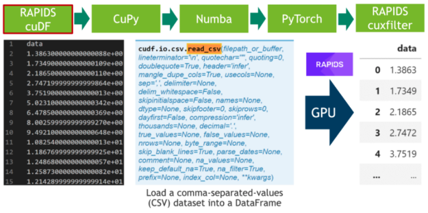
　　图 1 ：使用 RAPIDS CSV 解析器解析逗号分隔值（ CSV ）。

Step 1: Loading the data

We will start loading a CSV file containing 20 hours of heartbeats.

In [1]:

def retrieve_as_csv(url, root="./data"):

    # local import because we will never see them again ;)
    import os
    import urllib
    import zipfile
    import numpy as np
    from scipy.io import loadmat
    
    filename = os.path.join(root, 'ECG_one_day.zip')
        
    if not os.path.isdir(root):
        os.makedirs(root)
    if not os.path.isfile(filename):
        urllib.request.urlretrieve(url, filename)
                    
    with zipfile.ZipFile(filename, 'r') as zip_ref:
        zip_ref.extractall(root)
        
    stream = loadmat(os.path.join(root, 'ECG_one_day','ECG.mat'))['ECG'].flatten()
    
    csvname = os.path.join(root, 'heartbeats.csv')
    
    if not os.path.isfile(csvname):
        np.savetxt(csvname, stream[:-140000], delimiter=",", header="heartbeats", comments="")

# store the data as csv on disk
url = "https://www.cs.ucr.edu/~eamonn/ECG_one_day.zip"
retrieve_as_csv(url)

 

From the multiple libraries that can be used to read data from a CSV file (pandas, NumPy, …), we have chosen to use cuDF, a Python GPU-accelerated DataFrame library part of RAPIDS framework.

In [2]:

import cudf

heartbeats_cudf = cudf.read_csv("data/heartbeats.csv", dtype='float32')
heartbeats_cudf

Out[2]:

	heartbeats
0	-0.020
1	-0.010
2	-0.005
3	-0.005
4	-0.005
...	...
19999995	-0.005
19999996	0.015
19999997	0.005
19999998	-0.005
19999999	0.000

20000000 rows × 1 columns

 

Next, we will create a chart from the heartbeats_cudf DataFrame by making use of RAPIDS cuxfilter library.

We will get something similar to the following chart, but with a few nice features:

• The data is maintained in the GPU memory and operations like groupby aggregations, sorting and querying are done on the GPU itself, only returning the result as the output to the charts.
• The output is an interactive chart, facilitating data exploration.

In [3]:

import cuxfilter as cux
from cuxfilter.charts.datashader import line

# Chart width and height
WIDTH=600
HEIGHT=300

# 20 hours ECG look like a mess
heartbeats_cudf['x'] = heartbeats_cudf.index

line_cux = line(x='x', y='heartbeats', add_interaction=False)

_ = cux.DataFrame.from_dataframe(heartbeats_cudf).dashboard([line_cux])
line_cux.chart.title.text = 'ECG stream'
line_cux.chart.title.align = 'center'
line_cux.chart.width = WIDTH
line_cux.chart.height = HEIGHT
line_cux.view()[0]

 

Out[3]:

 

 

 

 

In [ ]:

　　步骤 2 ：数据分割

　　在下一步中，我们使用传统的信号处理技术将 20 小时的 ECG 分割成单个心跳。我们通过将 ECG 流与高斯分布的二阶导数（也称为里克尔小波）进行卷积来实现这一点，以便分离原型心跳中初始峰值的相应频带。使用 CuPy （一种 CUDA 加速的密集线性代数和阵列运算库）可以方便地进行小波采样和基于 FFT 的卷积运算。直接结果是，存储 ECG 数据的 RAPIDS cuDF 数据帧必须使用 DLPack 作为零拷贝机制转换为 CuPy 阵列。

　　

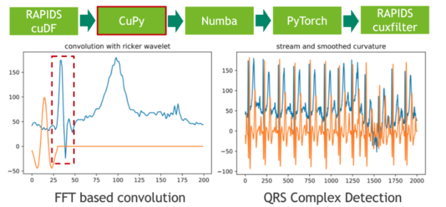
　　图 2 ：使用 CuPy 将 ele CTR 心图（ ECG ）流与固定宽度的 Ricker 小波卷积。

　　卷积的特征响应（结果）测量流中每个位置的固定频率内容的存在。请注意，我们选择小波的方式使局部最大值对应于心跳的初始峰值。

　　view rawCell040506.ipynb hosted with by GitHub

　　步骤 3 ：局部极大值检测

　　在下一步中，我们使用非最大抑制（ NMS ）的 1D 变体将这些极值点映射到二进制门。 NMS 确定流中每个位置的对应值是否为预定义窗口（邻域）中的最大值。这个令人尴尬的并行问题的 CUDA 实现非常简单。在我们的示例中，我们使用即时编译器 Numba 实现无缝的 Python 集成。 Numba 和 Cupy 都将 CUDA 阵列接口实现为零拷贝机制，因此可以完全避免从 Cupy 阵列到 Numba 设备阵列的显式转换。

　　

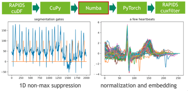
　　图 3 ：使用 Numba JIT 的 1D 非最大抑制和嵌入心跳。

　　每个心跳的长度是通过计算门位置的相邻差分（有限阶导数）来确定的。我们通过使用谓词门== 1 过滤索引域，然后调用 cupy 。 diff （）来实现这一点。得到的直方图描述了长度分布。

Inspecting heart beat lengths

The binary mask gate_cupy is 1 for each position that starts a heartbeat and 0 otherwise. Subsequently, we want to transform this dense representation with many zeroes to a sparse one where one only stores the indices in the stream that start a heartbeat. You could write a CUDA-kernel using warp-aggregated atomics for that purpose. In CuPy, however, this can be achieved easier by filtering the index domain with the predicate gate==1. An adjacent difference (discrete derivative cupy.diff) computes the heartbeat lengths as index distance between positive gate positions. Finally, the computed lengths are visualized in a histogram.

In [9]:

def indices_and_lengths_cupy(gate):

    # all indices 0 1 2 3 4 5 6 ...
    iota = cp.arange(len(gate))

    # after filtering with gate==1 it becomes 3 6 10
    indices = iota[gate == 1]
    lengths = cp.diff(indices)
    
    return indices, lengths

In [10]:

from cuxfilter.charts import bar

# inspect the segment lengths, we will later prune very long and short segments
indices_cupy, lengths_cupy = indices_and_lengths_cupy(gate_cupy)

# currently, cuxfilter doesn't support histogram chart with density=True,
# so we will create a histogram chart from a bar chart
BINS=30
lengths_hist_cupy = cp.histogram(lengths_cupy, bins=BINS, density=True)

hist_range = cp.max(lengths_cupy) - cp.min(lengths_cupy)
hist_width = int(hist_range/BINS)

lengths_cudf = cudf.DataFrame({'length': lengths_hist_cupy[0]})
lengths_cudf = lengths_cudf.loc[lengths_cudf.index.repeat(hist_width)]
lengths_cudf['x'] = cp.arange(0, BINS * hist_width) + cp.min(lengths_cupy)

bar_cux = bar(x='x', y='length', add_interaction=False)

_ = cux.DataFrame.from_dataframe(lengths_cudf).dashboard([bar_cux])
bar_cux.chart.title.text = 'Segment lengths'
bar_cux.chart.title.align = 'center'
bar_cux.chart.left[0].axis_label = ""
bar_cux.chart.width = WIDTH
bar_cux.chart.height = HEIGHT
bar_cux.view()[0]

 

Out[10]:

 

 

　　步骤 4 ：候选修剪和嵌入

　　我们打算使用固定长度的输入矩阵在心跳集上训练（卷积）变分自动编码器（ VAE ）。用 CUDA 内核可以实现心跳信号在零向量中的嵌入。在这里，我们再次使用 Numba 进行候选修剪和嵌入。

Candidate pruning and embedding in fixed length vectors

In a later stage we intend to train a Variational Autoencoder (VAE) with fixed-length input and thus the heartbeats must be embedded in a data matrix of fixed shape. According to the histogram the majority of length is somewhere in the range between 100 and 250. The embedding is accomplished with Numba kernel. A warp of 32 consecutive threads works on each heartbeat. The first thread in a warp (leader) checks if the heartbeat exhibits a valid length and increments a row counter in an atomic manner to determine the output row in the data matrix. Subsequently, the target row is communicated to the remaining 31 threads in the warp using the warp-intrinsic shfl_sync (broadcast). In a final step, we (re-)use the threads in the warp to write the values to the output row in the data matrix in a warp-cyclic fashion (warp-stride loop). Finally, we plot a few of the zero-embedded heartbeats and observe approximate alignment of the QRS complex -- exactly what we wanted to achieve.

In [11]:

@cuda.jit
def zero_padding_kernel(signal, indices, counter, lower, upper, out):
    """using warp intrinsics to speedup the calcuation"""
    
    for candidate in range(cuda.blockIdx.x, indices.shape[0]-1, cuda.gridDim.x):
        length = indices[candidate+1]-indices[candidate]
        
        # warp-centric: 32 threads process one signal
        if lower <= length <= upper:
            
            entry = 0
            if cuda.threadIdx.x == 0:
                # here we select in thread 0 what will be the target row
                entry = cuda.atomic.add(counter, 0, 1)
            
            # broadcast the target row to all other threads 
            # all 32 threads (warp) know the value
            entry = cuda.shfl_sync(0xFFFFFFFF, entry, 0)  
            
            for index in range(cuda.threadIdx.x, upper, 32):                
                out[entry, index] = signal[indices[candidate]+index] if index < length else 0.0
                
def zero_padding_numba(signal, indices, lengths, lower=100, upper=256):
    
    mask = (lower <= lengths) * (lengths <= upper)
    num_entries = int(cp.sum(mask))
    
    out = cp.empty((num_entries, upper), dtype=signal.dtype)
    counter = cp.zeros(1).astype(cp.int64)
    zero_padding_kernel[80*32, 32](signal, indices, counter, lower, upper, out)    
    cuda.synchronize()
    
    print("removed", 100-100*num_entries/len(lengths), "percent of the candidates")
    
    return out

# let's prune the short and long segments (heartbeats) and normalize them
data_cupy = zero_padding_numba(heartbeats_cupy, indices_cupy, lengths_cupy, lower=100, upper=256)    

 

removed 3.3824004429883274 percent of the candidates

In [12]:

# looks good, they are approximately aligned

HEARTBEATS_SAMPLE = 10
data_cudf = cudf.DataFrame({'y_{}'.format(i):data_cupy[i] for i in range(HEARTBEATS_SAMPLE)})
data_cudf['x'] = cp.arange(0, data_cupy.shape[1])
data_cudf = data_cudf.astype('float64')


stacked_lines_cux = stacked_lines(x='x', y=['y_{}'.format(i) for i in range(HEARTBEATS_SAMPLE)],
                                  legend=False, add_interaction=False,
                                  colors = ["red", "grey", "black", "purple", "pink",
                                            "yellow", "brown", "green", "orange", "blue"])
                                  

_ = cux.DataFrame.from_dataframe(data_cudf).dashboard([stacked_lines_cux])
stacked_lines_cux.chart.title.text = 'A few heartbeats'
stacked_lines_cux.chart.title.align = 'center'
stacked_lines_cux.chart.width = WIDTH
stacked_lines_cux.chart.height = HEIGHT
stacked_lines_cux.view()[0]

 

Out[12]:

 

 

 

　　步骤 5 ：异常值检测

　　在这一步中，我们在 75% 的数据上训练 VAE 模型。 DLPack 再次用作零拷贝机制，将 CuPy 数据矩阵映射到 PyTorch 张量。

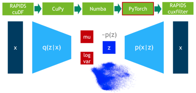
　　图 4 ：使用 PyTorch 训练可变自动编码器。

Installing PyTorch...
WARNING: Running pip as root will break packages and permissions. You should install packages reliably by using venv: https://pip.pypa.io/warnings/venv

 

Subsequently, we define the network topology. Here, we use a convolutional version but you could also experiment with a classical MLP VAE.

In [14]:

import torch

class Swish(torch.nn.Module):    

    def __init__(self):
        super().__init__()        
        self.alpha = torch.nn.Parameter(torch.tensor([1.0], requires_grad=True))
    
    def forward(self, x):
        return x*torch.sigmoid(self.alpha.to(x.device)*x)

class Downsample1d(torch.nn.Module):    
    
    def __init__(self):
        super().__init__()
        
        self.filter = torch.tensor([1.0, 2.0, 1.0]).view(1, 1, 3)
    
    def forward(self, x):
        w = torch.cat([self.filter]*x.shape[1], dim=0).to(x.device)
        return torch.nn.functional.conv1d(x, w, stride=2, padding=1, groups=x.shape[1])

class LightVAE(torch.nn.Module):
    def __init__(self, num_dims):
        super(LightVAE, self).__init__()
        
        self.num_dims = num_dims
        assert num_dims & num_dims-1 == 0, "num_dims must be power of 2"
        
        self.down   = Downsample1d()
        self.up     = torch.nn.Upsample(scale_factor=2)
        self.sigma  = Swish()
        
        self.conv0  = torch.nn.Conv1d(1, 2, kernel_size=3, stride=1, padding=1)
        self.conv1  = torch.nn.Conv1d(2, 4, kernel_size=3, stride=1, padding=1)
        self.conv2  = torch.nn.Conv1d(4, 8, kernel_size=3, stride=1, padding=1)
        self.convA  = torch.nn.Conv1d(8, 2, kernel_size=3, stride=1, padding=1)
        self.convB  = torch.nn.Conv1d(8, 2, kernel_size=3, stride=1, padding=1)

        self.restore = torch.nn.Linear(2, 8*num_dims//8)
        
        self.conv3  = torch.nn.Conv1d( 8, 4, kernel_size=3, stride=1, padding=1)
        self.conv4  = torch.nn.Conv1d( 4, 2, kernel_size=3, stride=1, padding=1)
        self.conv5  = torch.nn.Conv1d( 2, 1, kernel_size=3, stride=1, padding=1)
        
    def encode(self, x):
        
        x  = x.view(-1, 1, self.num_dims)
        x  = self.down(self.sigma(self.conv0(x)))
        x  = self.down(self.sigma(self.conv1(x)))
        x  = self.down(self.sigma(self.conv2(x)))
        
        return torch.mean(self.convA(x), dim=(2,)), \
               torch.mean(self.convB(x), dim=(2,))

    def reparameterize(self, mu, logvar):
        
        std = torch.exp(0.5*logvar)
        eps = torch.randn_like(std)
        
        return mu + eps*std

    def decode(self, z):
        
        x = self.restore(z).view(-1, 8, self.num_dims//8)
        x = self.sigma(self.conv3(self.up(x)))
        x = self.sigma(self.conv4(self.up(x)))   
              
        return self.conv5(self.up(x)).view(-1, self.num_dims)

    def forward(self, x):
        mu, logvar = self.encode(x)
        z = self.reparameterize(mu, logvar)
        return self.decode(z), mu, logvar
    
# Reconstruction + KL divergence losses summed over all elements and batch
def loss_function(recon_x, x, mu, logvar):
    MSE = torch.sum(torch.mean(torch.square(recon_x-x), dim=1))

    # see Appendix B from VAE paper:
    # Kingma and Welling. Auto-Encoding Variational Bayes. ICLR, 2014
    # https://arxiv.org/abs/1312.6114
    # 0.5 * sum(1 + log(sigma^2) - mu^2 - sigma^2)
    KLD = -0.1 * torch.sum(torch.mean(1 + logvar - mu.pow(2) - logvar.exp(), dim=1))

    return MSE + KLD

 

Pytorch expects its dedicated tensor type and thus we need to map the CuPy array data_cupy to a FloatTensor. We perform that again using zero-copy functionality via DLPack. The remaining code is plain Pytorch program that trains the VAE on the training set for 10 epochs using the Adam optimizer.

In [15]:

# zero-copy to pytorch tensors using dlpack
from torch.utils import dlpack

cp.random.seed(42)
cp.random.shuffle(data_cupy)

split = int(0.75*len(data_cupy))
trn_torch = dlpack.from_dlpack(data_cupy[:split].toDlpack())
tst_torch = dlpack.from_dlpack(data_cupy[split:].toDlpack())

dim = trn_torch.shape[1]
model = LightVAE(dim).to('cuda')
optimizer = torch.optim.Adam(model.parameters())

In [16]:

# let's train a VAE
NUM_EPOCHS = 10
BATCH_SIZE = 1024

trn_loader = torch.utils.data.DataLoader(trn_torch, batch_size=BATCH_SIZE, shuffle=True)
tst_loader = torch.utils.data.DataLoader(tst_torch, batch_size=BATCH_SIZE, shuffle=False)

model.train()
for epoch in range(NUM_EPOCHS):
    trn_loss = 0.0
    for data in trn_loader:
        optimizer.zero_grad()
        recon_batch, mu, logvar = model(data)
        loss = loss_function(recon_batch, data, mu, logvar)
        loss.backward()
        trn_loss += loss.item()
        optimizer.step()
       
    print('====> Epoch: {} Average loss: {:.4f}'.format(
          epoch, trn_loss / len(trn_loader.dataset)))

 

====> Epoch: 0 Average loss: 0.0186
====> Epoch: 1 Average loss: 0.0077
====> Epoch: 2 Average loss: 0.0066
====> Epoch: 3 Average loss: 0.0063
====> Epoch: 4 Average loss: 0.0061
====> Epoch: 5 Average loss: 0.0060
====> Epoch: 6 Average loss: 0.0059
====> Epoch: 7 Average loss: 0.0059
====> Epoch: 8 Average loss: 0.0058
====> Epoch: 9 Average loss: 0.0058

　　步骤 6 ：结果可视化

　　在最后一步中，我们可视化剩余 25% 数据的潜在空间。

　　

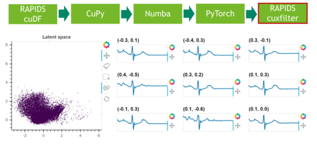
　　图 5 ：使用 RAPIDS cuxfilter 对潜在空间进行采样和可视化。

Let's check if the test loss is in the same range:

In [17]:

# it will be used to visualize a scatter char
mu_cudf = cudf.DataFrame()

model.eval()
with torch.no_grad():
    tst_loss = 0
    for data in tst_loader:
        recon_batch, mu, logvar = model(data)
        tst_loss += loss_function(recon_batch, data, mu, logvar).item()
        mu_cudf = mu_cudf.append(cudf.DataFrame(mu, columns=['x', 'y']))
            
tst_loss /= len(tst_loader.dataset)
print('====> Test set loss: {:.4f}'.format(tst_loss))

 

====> Test set loss: 0.0074

 

Finally, we visualize the latent space which is an approximate isotropic Gaussian centered around the origin:

In [18]:

from cuxfilter.charts import scatter
    
scatter_chart_cux = scatter(x='x', y='y', pixel_shade_type="linear",
                            legend=False, add_interaction=False)
    
_ = cux.DataFrame.from_dataframe(mu_cudf).dashboard([scatter_chart_cux])
scatter_chart_cux.chart.title.text = 'Latent space'
scatter_chart_cux.chart.title.align = 'center'
scatter_chart_cux.chart.width = WIDTH
scatter_chart_cux.chart.height = 2*HEIGHT
scatter_chart_cux.view()[0]

 

 

 

 

 

Out[18]:

 

 

 

 

　　结论

　　从这篇和前面的博文中可以看出，互操作性对于设计高效的数据管道至关重要。在不同的框架之间复制和转换数据是一项昂贵且极其耗时的任务，它为数据科学管道增加了零价值。数据科学工作负载变得越来越复杂，多个软件库之间的交互是常见的做法。 DLPack 和 CUDA 阵列接口是事实上的数据格式标准，保证了基于 GPU 的框架之间的零拷贝数据交换。

　　对外部内存管理器的支持是一个很好的特点，在评估您的管道将使用哪些软件库时要考虑。例如，如果您的任务同时需要数据帧和数组数据操作，那么最好选择 RAPIDS cuDF + CuPy 库。它们都受益于 GPU 加速，支持 DLPack 以零拷贝方式交换数据，并共享同一个内存管理器 RMM 。或者， RAPIDS cuDF + JAX 也是一个很好的选择。然而，后一种组合 或许需要额外的开发工作来利用内存使用，因为 JAX 缺乏对外部内存分配器的支持。

　　在处理大型数据集时，数据加载和数据传输瓶颈经常出现。 NVIDIA GPU 直接技术起到了解救作用，它支持将数据移入或移出 GPU 内存，而不会加重 CPU 的负担，并将不同节点上 GPU 之间传输数据时所需的数据副本数量减少到一个。

　　关于作者

　　Christian Hundt 在德国美因茨的 Johannes Gutenberg 大学（ JGU ）获得了理论物理的文凭学位。在他的博士论文中，他研究了时间序列数据挖掘算法在大规模并行架构上的并行化。作为并行和分布式体系结构组的博士后研究员，他专注于各种生物医学应用的高效并行化，如上下文感知的元基因组分类、基因集富集分析和胸部 mri 的深层语义图像分割。他目前的职位是深度学习解决方案架构师，负责协调卢森堡的 NVIDIA 人工智能技术中心（ NVAITC ）的技术合作。

　　Miguel Martinez 是 NVIDIA 的高级深度学习数据科学家，他专注于 RAPIDS 和 Merlin 。此前，他曾指导过 Udacity 人工智能纳米学位的学生。他有很强的金融服务背景，主要专注于支付和渠道。作为一个持续而坚定的学习者， Miguel 总是在迎接新的挑战。

　　审核编辑：郭婷