

时序分析实战之SARIMA、Linear model介绍
描述
1 数据准备
首先引入相关的 statsmodels,包含统计模型函数(时间序列)。
# 引入相关的统计包
import warnings  # 忽略警告
warnings.filterwarnings('ignore')

import numpy as np  # 矢量和矩阵
import pandas as pd  # 表格和数据操作
import matplotlib.pyplot as plt
import seaborn as sns
from dateutil.relativedelta import relativedelta  # 有风格地处理日期
from scipy.optimize import minimize  # 函数优化
import statsmodels.formula.api as smf  # 统计与经济计量
import statsmodels.tsa.api as smt
import scipy.stats as scs
from itertools import product
from tqdm import tqdm_notebook
import statsmodels.api as sm
用真实的手机游戏数据作为样例,研究每小时观看的广告数和每日所花的游戏币。
# 1 如真实的手机游戏数据,将调查每小时观看的广告和每天花费的游戏币
ads = pd.read_csv(r'./test/ads.csv', index_col=['Time'], parse_dates=['Time'])
currency = pd.read_csv(r'./test/currency.csv', index_col=['Time'], parse_dates=['Time'])
2 稳定性
建模前,先来了解一下稳定性(stationarity)。
如果一个过程是平稳的,这意味着它不会随时间改变其统计特性,如均值和方差等等。
方差的恒常性称为同方差,协方差函数不依赖于时间,它只取决于观测值之间的距离。
非平稳过程是指分布参数或者分布规律随时间发生变化。也就是说,非平稳过程的统计特征是时间的函数(随时间变化)。
下面的红色图表不是平稳的:
- 平均值随时间增加
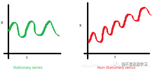
- 方差随时间变化

- 随着时间的增加,距离变得越来越近。因此,协方差不是随时间而恒定的

为什么平稳性如此重要呢? 通过假设未来的统计性质与目前观测到的统计性质不会有什么不同,可以很容易对平稳序列进行预测。
大多数的时间序列模型,以这样或那样的方式,试图预测那些属性(例如均值或方差)。
如果原始序列不是平稳的,那么未来的预测将是错误的。
大多数时间序列都是非平稳的,但可以(也应该)改变这一点。
平稳时间序列的类型:
- 平稳过程(stationary process):产生平稳观测序列的过程。
- 平稳模型(stationary model):描述平稳观测序列的模型。
- 趋势平稳(trend stationary):不显示趋势的时间序列。
- 季节性平稳(seasonal stationary):不表现出季节性的时间序列。
- 严格平稳(strictly stationary):平稳过程的数学定义,特别指观测值的联合分布不受时移的影响。
若时序中有明显的趋势和季节性,则对这些成分建模,将它们从观察中剔除,然后用残差训练建模。
平稳性检查方法(可以检查观测值和残差):
- 看图:绘制时序图,看是否有明显的趋势或季节性,如绘制频率图,看是否呈现高斯分布(钟形曲线)。
- 概括统计:看不同季节的数据或随机分割或检查重要的差分,如将数据分成两部分,计算各部分的均值和方差,然后比较是否一样或同一范围内
- 统计测试:选用统计测试检查是否有趋势和季节性
若时序的均值和方差相差过大,则有可能是非平稳序列,此时可以对观测值取对数,将指数变化转变为线性变化。然后再次查看取对数后的观测值的均值和方差以及频率图。
上面前两种方法常常会欺骗使用者,因此更好的方法是用统计测试 sm.tsa.stattools.adfuller()。
接下来将学习如何检测稳定性,从白噪声开始。
# 5经济计量方法(Econometric approach)
# ARIMA 属于经济计量方法
# 创建平稳序列
white_noise = np.random.normal(size=1000)
with plt.style.context('bmh'):
    plt.figure(figsize=(15,5))
    plt.plot(white_noise)

标准正态分布产生的过程是平稳的,在0附近振荡,偏差为1。现在,基于这个过程将生成一个新的过程,其中每个后续值都依赖于前一个值。
def plotProcess(n_samples=1000,rho=0):
    x=w=np.random.normal(size=n_samples)
    for t in range(n_samples):
        x[t] = rho*x[t-1]+w[t]

    with plt.style.context('bmh'):
        plt.figure(figsize=(10,5))
        plt.plot(x)
        plt.title('Rho {}\\n Dickey-Fuller p-value: {}'.format(rho,round(sm.tsa.stattools.adfuller(x)[1],3)))

#-------------------------------------------------------------------------------------
for rho in [0,0.6,0.9,1]:
    plotProcess(rho=rho)


第一张图与静止白噪声一样。
第二张图,ρ增加至0.6,大的周期出现,但整体是静止的。
第三张图,偏离0均值,但仍然在均值附近震荡。
第四张图,ρ= 1,有一个随机游走过程即非平稳时间序列。当达到临界值时, 不返回其均值。从两边减去 ,得到 ,左边的表达式被称为 一阶差分 。
如果 ρ= 1,那么一阶差分等于平稳白噪声 。这是 Dickey-Fuller时间序列平稳性测试 (测试单位根的存在)背后的主要思想。
如果 可以用一阶差分从非平稳序列中得到平稳序列,称这些序列为1阶积分 。 该检验的零假设是时间序列是非平稳的 ,在前三个图中被拒绝,在最后一个图中被接受。
1阶差分并不总是得到一个平稳的序列,因为这个过程可能是 d 阶的积分,d > 1阶的积分(有多个单位根)。在这种情况下,使用增广的Dickey-Fuller检验,它一次检查多个滞后时间。
可以使用不同的方法来去除非平稳性:各种顺序差分、趋势和季节性去除、平滑以及转换如Box-Cox或对数转换。
3 SARIMA
接下来开始建立ARIMA模型,在建模之前需要将非平稳时序转换为平稳时序。
3.1 去除非稳定性
摆脱非平稳性,建立SARIMA(Getting rid of non-stationarity and building SARIMA)
def tsplot(y,lags=None,figsize=(12,7),style='bmh'):
"""
Plot time series, its ACF and PACF, calculate Dickey-Fuller test
y:timeseries
lags:how many lags to include in ACF,PACF calculation
"""
ifnot isinstance(y, pd.Series):
y = pd.Series(y)
with plt.style.context(style):
     fig = plt.figure(figsize=figsize)
     layout=(2,2)
     ts_ax = plt.subplot2grid(layout, (0,0), colspan=2)
     acf_ax = plt.subplot2grid(layout, (1,0))
     pacf_ax = plt.subplot2grid(layout, (1,1))

     y.plot(ax=ts_ax)
     p_value = sm.tsa.stattools.adfuller(y)[1]
     ts_ax.set_title('Time Series Analysis Plots\\n Dickey-Fuller: p={0:.5f}'.format(p_value))
     smt.graphics.plot_acf(y,lags=lags, ax=acf_ax)
     smt.graphics.plot_pacf(y,lags=lags, ax=pacf_ax)
     plt.tight_layout()
#-------------------------------------------------------------------------------------
tsplot(ads.Ads, lags=60)

从图中可以看出,Dickey-Fuller检验拒绝了单位根存在的原假设(p=0);序列是平稳的,没有明显的趋势,所以均值是常数,方差很稳定。
唯一剩下的是季节性,必须在建模之前处理它。可以通过季节差分去除季节性,即序列本身减去一个滞后等于季节周期的序列。
ads_diff = ads.Ads-ads.Ads.shift(24) # 去除季节性
tsplot(ads_diff[24:], lags=60)

ads_diff = ads_diff - ads_diff.shift(1) # 去除趋势
tsplot(ads_diff[24+1:], lags=60) # 最终图


第一张图中,随着季节性的消失,自回归好多了,但是仍存在太多显著的滞后,需要删除。首先使用一阶差分,用滞后1从自身中减去时序。
第二张图中,通过季节差分和一阶差分得到的序列在0周围震荡。Dickey-Fuller试验表明,ACF是平稳的,显著峰值的数量已经下降,可以开始建模了。
3.2 建 SARIMA 模型
SARIMA:Seasonal Autoregression Integrated Moving Average model。
是简单自回归移动平均的推广,并增加了积分的概念。
- AR (p): 利用一个观测值和一些滞后观测值之间的依赖关系的模型。模型中的最大滞后称为p。要确定初始p,需要查看PACF图并找到最大的显著滞后,在此之后大多数其他滞后都变得不显著。
- I (d): 利用原始观测值的差值(如观测值减去上一个时间步长的观测值)使时间序列保持平稳。这只是使该系列固定所需的非季节性差分的数量。在例子中它是1,因为使用了一阶差分。
- MA (q):利用观测值与滞后观测值的移动平均模型残差之间的相关性的模型。目前的误差取决于前一个或前几个,这被称为q。初始值可以在ACF图上找到,其逻辑与前面相同
每个成分都对应着相应的参数。
SARIMA(p,d,q)(P,D,Q,s) 模型需要选择趋势和季节的超参数。
趋势参数 ,趋势有三个参数,与ARIMA模型的参数一样:
- p: 模型中包含的滞后观测数,也称滞后阶数。
- d: 原始观测值被差值的次数,也称为差值度。
- q:移动窗口的大小,也叫移动平均的阶数
季节参数 :
- S(s):负责季节性,等于单个季节周期的时间步长
- P:模型季节分量的自回归阶数,可由PACF推导得到。但是需要看一下显著滞后的次数,是季节周期长度的倍数。如果周期等于24,看到24和48的滞后在PACF中是显著的,这意味着初始P应该是2。P=1将利用模型中第一次季节偏移观测,如t-(s*1)或t-24;P=2,将使用最后两个季节偏移观测值t-(s * 1), t-(s * 2)
- Q:使用ACF图实现类似的逻辑
- D:季节性积分的阶数(次数)。这可能等于1或0,取决于是否应用了季节差分。
可以通过分析ACF和PACF图来选择趋势参数,查看最近时间步长的相关性(如1,2,3)。
同样,可以分析ACF和PACF图,查看季节滞后时间步长的相关性来指定季节模型参数的值。
现在知道了如何设置初始参数,查看最终图并设置参数。
上面倒数第一张图就是最终图:
- p:最可能是4,因为它是PACF上最后一个显著的滞后,在这之后,大多数其他的都不显著。
- d:为1,因为我们计算了一阶差分
- q:应该在4左右,就像ACF上看到的那样
- P:可能是2,因为24和48的滞后对PACF有一定的影响
- D:为1,因为计算了季节差分
- Q:可能1,ACF的第24个滞后显著,第48个滞后不显著。
下面看不同参数的模型表现如何:
# 建模 SARIMA
# setting initial values and some bounds for them
ps = range(2,5)
d=1
qs=range(2,5)
Ps=range(0,2)
D=1
Qs=range(0,2)
s=24#season length

# creating list with all the possible combinations of parameters
parameters=product(ps,qs,Ps,Qs)
parameters_list = list(parameters)
print(parameters)
print(parameters_list)
print(len(parameters_list))
# 36
def optimizeSARIMA(parameters_list, d,D,s):
    """
    Return dataframe with parameters and corresponding AIC
    parameters_list:list with (p,q,P,Q) tuples
    d:integration order in ARIMA model
    D:seasonal integration order
    s:length of season
    """
    results = []
    best_aic = float('inf')

    for param in tqdm_notebook(parameters_list):
        # we need try-exccept because on some combinations model fails to converge
        try:
            model = sm.tsa.statespace.SARIMAX(ads.Ads, order=(param[0], d,param[1]),
                                              seasonal_order=(param[2], D,param[3], s)).fit(disp=-1)
        except:
            continue
        aic = model.aic
        # saving best model, AIC and parameters
        if aic< best_aic:
            best_model = model
            best_aic = aic
            best_param = param
        results.append([param, model.aic])

    result_table = pd.DataFrame(results)
    result_table.columns = ['parameters', 'aic']
    # sorting in ascending order, the lower AIC is - the better
    result_table = result_table.sort_values(by='aic',ascending=True).reset_index(drop=True)

    return result_table
%%time
result_table = optimizeSARIMA(parameters_list, d,D,s)

result_table.head()

# set the parameters that give the lowerst AIC
p,q,P,Q = result_table.parameters[0]
best_model = sm.tsa.statespace.SARIMAX(ads.Ads, order=(p,d,q),seasonal_order=(P,D,Q,s)).fit(disp=-1)
print(best_model.summary()) # 打印拟合模型的摘要。这总结了所使用的系数值以及对样本内观测值的拟合技巧。

# inspect the residuals of the model
tsplot(best_model.resid[24+1:], lags=60)
parameters          aic
0  (2, 3, 1, 1)  3888.642174
1  (3, 2, 1, 1)  3888.763568
2  (4, 2, 1, 1)  3890.279740
3  (3, 3, 1, 1)  3890.513196
4  (2, 4, 1, 1)  3892.302849

                                Statespace Model Results
==========================================================================================
Dep. Variable:                                Ads   No. Observations:                  216
Model:             SARIMAX(2, 1, 3)x(1, 1, 1, 24)   Log Likelihood               -1936.321
Date:                            Sun, 08 Mar 2020   AIC                           3888.642
Time:                                    23:06:23   BIC                           3914.660
Sample:                                09-13-2017   HQIC                          3899.181
                                     - 09-21-2017
Covariance Type:                              opg
==============================================================================
                 coef    std err          z      P  >|z|      [0.0250.975]
------------------------------------------------------------------------------
ar.L1          0.79130.2702.9280.0030.2621.321
ar.L2         -0.55030.306-1.7990.072-1.1500.049
ma.L1         -0.73160.262-2.7930.005-1.245-0.218
ma.L2