过滤器选择＆amp;设计：系统性能的网关

All too often, designers spend so much time focusing on the specification and selection of their complex, higher cost devices such as processors, FPGAs, and ADCs, that they don’t fully take into account the major performance impacts, as well as cost and power issues, that are driven by the selection and integration of so-called “low-end” components such as filters.
In fact, the specification and design of filter circuitry can often be among the most important factors that determine overall system success. For instance, if the filtering design in a relatively low-bandwidth application fails to eliminate high-bandwidth noise at the front-end of the signal chain, the system has to burn extra power just to propagate that unwanted noise down the signal chain. Or, when processing signals of a certain bandwidth, such as in a channel-based radio receiver, an inadequate filtering design can lead to unnecessary processing of signals from adjacent channels. This leads to a waste of power and a potential degradation of the target signal.
Proper filter design also prevents the signal path from contributing noise to other parts of the system, such as keeping high-frequency signals from coupling back into the power circuit and causing instability or fluctuations. In essence, bypass capacitors are actually the simplest category of analog filters and are widely used in all types of designs.
Below is a brief overview of the role of filters, the types of filters, and differences between digital and analog approaches as well as between passive and active filtering designs. Then there are some specific design tips for simulating and selecting analog filters for an example application to drive high-performance analog-digital converters (ADCs).
The role of filters
Filters are electronic signal processing circuits that are aimed at removing unwanted frequency components from the signal, enhancing wanted signals, or both.
Electronic filters generally can be grouped into the following categories:

• High-pass filters—attenuation of frequencies below the cut-off points.
• Low-pass filters—attenuation of frequencies above the cut-off points.
• Band-pass filters—attenuation of frequencies both above and below the target frequency band.
• Notch filters—attenuation of certain frequencies while allowing all others to pass.

The frequency response of a filter is typically characterized in terms of Bode Plots, which express amplitude gain in decibels and phase in radians or degrees. The bandwidth, Δf, of a filter is defined as energy versus frequency. The Q factor of the filter is defined by f0/Δf where f0 is the center frequency of a bandpass filter and Δf is the bandwidth. See Figure 2 for example curves. The higher the Q, the narrower and ‘sharper’ the peak will be. In essence, the Q-factor is a measure of ‘quality’ for a particular resonance point on the frequency spectrum. Depending on the specific application requirements, there are a number of different filter configurations that can be considered to provide alternatives with regard to optimizing the Q factor, the filter’s stability and other key characteristics.
These configurations include the following:

• Chebyshev filter—slight peaking/ripple in the passband before the corner; Q>0.7071 for 2nd-order filters.
• Butterworth filter—flattest amplitude response; Q=0.7071 for 2nd-order filters.
• Linkwitz–Riley filter—desirable properties for audio crossover applications; Q = 0.5 (critically damped).
• Bessel filter—best time-delay, best overshoot response; Q=0.577 for 2nd-order filters.
• Paynter or transitional Thompson-Butterworth or “compromise” filter—faster fall-off than Bessel; Q=0.639 for 2nd-order filters.
• Elliptic filter or Cauer filter—add a notch (or “zero”) just outside the passband, to give a much greater slope in this region than the combination of order and damping factor without the notch.

Digital filters
Digital filters sample discrete time signals and need to operate on digital inputs in order to provide digital outputs. Digital filtering is a more complex approach than analog and is typically used in conjunction with FPGAs or microcontrollers, where there is already a significant amount of programming, digital gates, et cetera. Because the signals in these systems need to be digitized to go into the FPGA or microprocessor anyway, it is not a major cost to the system to digitize the signals first and then conduct filtering within the digital processing chain.
A digital filter usually consists of an analog-to-digital converter to sample the input signal, followed by a microprocessor and some peripheral components such as memory for tasks like storing data and filtering coefficients. In a typical digital filtering application, software running on a digital signal processor (DSP) reads input samples from an A/D converter, performs the mathematical manipulations dictated by theory for the required filter type, and outputs the result via a D/A converter. In mathematical terms, filtering is in essence the multiplication of the signal spectrum by the frequency domain impulse response of the filter. For an ideal lowpass filter, the passband part of the signal spectrum is multiplied by one and the stopband part of the signal by zero.
In addition to adding complexity, digital filters generally consume more power than analog approaches. Also, because digital filters use a sampling process and discrete-time processing, there is an inherent latency factor, which must be taken into account with regard to overall design objectives. Digital filter designs can be simplified by limiting the number of bits used, depending on the accuracy requirements of the application.
Digital filters are most often used in systems that require complex signal management and/or a high degree of precision. Because these designs digitize the signal before they perform operations on it, they offer a great degree of flexibility for complex mathematical functions. This makes it very easy to change the coefficient in order to tune the filter for the desired output, such as in a Finite Impulse Response (FIR) filter design.
Analog filters
Analog filters are used to process continuous-time signals and work directly on analog inputs, typically providing a near instantaneous response from input to output. In the ideal case, an analog filter would provide 100 percent transmission within the specified frequency passband and 100 percent attenuation outside of that passband. However, in the real world, analog filters can only approximate this ideal performance, with some attenuation in the passband and less than 100 percent attenuation over the stopband frequency range. Analog is generally the preferred solution when the design’s filtering requirements are relatively simple, and especially if minimizing system cost and/or power consumption is an important factor.
Filter Type Characteristics Application Areas Digital Filters

• Digital inputs & digital outputs
• Higher complexity
• Greater flexibility

• FPGA & microprocessor based systems
• High-precision, complex filtering
  requirements

Analog Filters

• Analog inputs & analog outputs
• Lower cost
• Lower power

• Analog-only signal chains
• Front-end filtering in
  mixed-signal designs

Figure 1: Comparison of digital and analog filtering approaches.
Passive vs. active
If a very precise filter is required, designers may build it from scratch using all passive components. However, the cost, space, and complexity can often become prohibitive, so where possible, most designs lean toward an active filter approach using a combination of op amps and passives. This section provides a very brief overview of the differences and the tradeoffs between passive and active filter approaches.
By definition, a passive filter is made only from passive elements. It does not require an external power source beyond the signal itself. Since most filters are linear, passive filters are typically composed of just the four basic linear elements—resistors, capacitors, inductors, and transformers. More complex passive filters may involve nonlinear elements, or more complex linear elements, such as transmission lines.
A passive filter has several advantages over an active filter:

• Guaranteed stability.
• Passive filters scale better to large signals (tens of amperes, hundreds of volts).
• No power consumption.
• May be less expensive in discrete designs (unless large coils are required).

Passive filters are commonly used in applications involving higher voltage and current levels, such as speaker crossover designs, filters in power distribution networks and power supplies. Passive filters are uncommon in monolithic integrated circuit designs, where active devices are inexpensive compared to resistors and capacitors, and inductors are prohibitively expensive.
Active filters are implemented using a combination of passive and active (amplifying) components, and require an outside power source. Operational amplifiers are frequently used in active filter designs. These can have high Q factor, and can achieve resonance without the use of inductors. However, their upper frequency limit is limited by the bandwidth of the amplifiers used.
Active filters have three main advantages over passive filters:

• Inductors can be avoided. Passive filters cannot obtain a high Q without inductors but they are large and expensive at low frequencies, have significant internal resistance, and may pick up surrounding electromagnetic signals.
• The shape of the response, the Q factor, and the tuned frequency can be set simply by varying resistors and one parameter can often be adjusted without affecting the others.
• The amplifier powering the filter can also be used to buffer the filter from the electronic components it drives or is fed from, thereby eliminating variations that could affect the shape of the frequency response.

Design example: Modeling an active filter for high-performance ADCs
When creating any mixed-signal system, the first thing that the designer typically chooses is the ADC because the system needs a certain number of bits, as well as a specified speed and sampling frequency. Once the ADC has been selected, everything else in the supporting circuitry is aimed at driving the ADC to the optimal specifications, without degrading performance. It is critical that the op amps and other components in the filter circuit provide high-speed signal processing without adding to the noise floor in order for the ADC to run as close as possible to its maximum specified dynamic range or resolution.
To model the specifics for implementing an active filter, engineers need simulation tools that can take the target filter shape and deliver a set of op amps and external passives that accurately achieve the desired filter response. There are a number of such tools available online but it’s important to keep in mind the key differences between modeling with ideal specifications versus modeling for real-world production. Most tools estimate amplifier frequency response with a single-pole approximation instead of taking into account the second and third order effects present in commercial amps. When filters were designed for low frequencies and the amplifiers had abundant bandwidth compared to the application, this was a reasonable estimation. This is no longer true and a better simulation tool is crucial. One such comprehensive simulation tool can be accessed at web.transim.com/iSimFilter
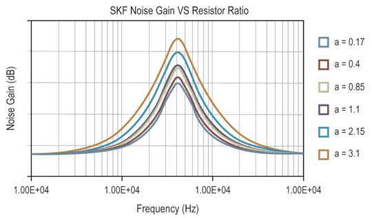
It is also imperative that the model simulation goes beyond specifying just the op amps and also models the various resistors and capacitors needed to complete an optimal filter circuit for the specific application. For example, Figure 2 shows a simulation from the iSimFilter tool that models noise gain in dB for various resistor levels. The Sallen-Key filter (SKF) used in this example is an electronic filter topology used to implement second-order active filters (the ‘alpha’ values listed represent the ratio of feedback resistor to gain resistors).

Figure 2: iSimFilter modeling of Sallen-Key filter noise for various resistor levels.
In our specific design example for driving a high-speed ADC, such as the 500 MSPS ISLA112P50 12-bit and the ISLA214P50 14-bit ADCs, the recommended op amp solution is the ISL55210, which operates at very low power (115 mW) and has negligible noise with respect to the ADC. Therefore, adding gain and filtering has virtually no impact on the system SFDR. The ISL55210 features very high slew rates, low noise, ultra-low distortion, and provides a 4 GHz gain bandwidth with input noise of only 0.85 nV/√Hz and consistent performance over a wide temperature and gain range. The op amp suppresses even-order harmonic distortion, which is usually caused by asymmetrical or unbalanced signal paths, and supports gains greater than two with minimal bandwidth or SFDR degradation.
Figure 3 illustrates a typical filter design using the ISL55210 and passives support circuitry to drive a 12-bit ISLA112P50 ADC.

Figure 3: Filter design with ISL55210 and support circuitry.
Summary
Filtering may seem to be a simple design issue, and therefore it doesn’t always get the attention that it deserves. But filter circuits actually are the “sentinels at the gateway” to the signal path and are critical for achieving full performance in the higher-cost devices that form the heart of the overall system.
Proper selection, modeling, and integration of the op amps, passives, and other elements of the filtering circuitry can make or break the success of the overall design. Even the most advanced ADCs, processors, and other high-end devices become a waste of money if they can’t be driven as close as possible to their optimal specification levels.