如何搭建自己的神经网络

神经网络基本概念

（1）激励函数：

例如一个神经元对猫的眼睛敏感，那当它看到猫的眼睛的时候，就被激励了，相应的参数就会被调优，它的贡献就会越大。

下面是几种常见的激活函数：

x轴表示传递过来的值，y轴表示它传递出去的值：

 

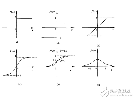
激励函数在预测层，判断哪些值要被送到预测结果那里：

 

TensorFlow 常用的 activation function

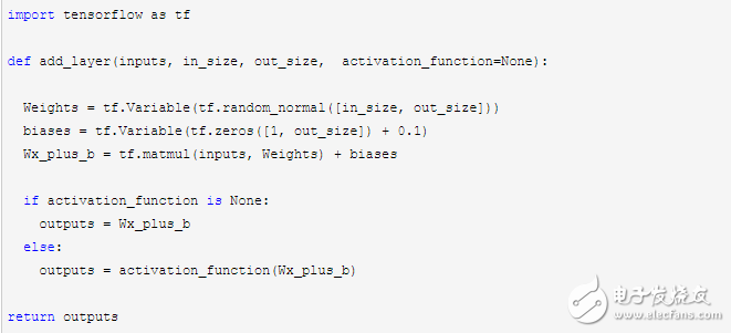
（2）添加神经层：

输入参数有 inputs， in_size， out_size， 和 activation_function

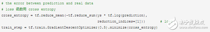
分类问题的 loss 函数 cross_entropy ：

 

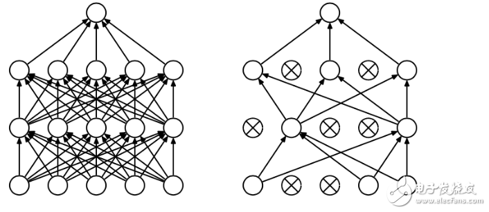
overfitting：

下面第三个图就是 overfitting，就是过度准确地拟合了历史数据，而对新数据预测时就会有很大误差：

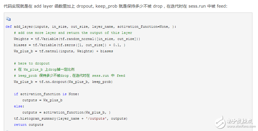
Tensorflow 有一个很好的工具， 叫做dropout， 只需要给予它一个不被 drop 掉的百分比，就能很好地降低 overfitting。

dropout 是指在深度学习网络的训练过程中，按照一定的概率将一部分神经网络单元暂时从网络中丢弃，相当于从原始的网络中找到一个更瘦的网络，这篇博客中讲的非常详细

 

 

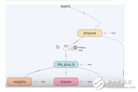
5. 可视化 Tensorboard

Tensorflow 自带 tensorboard ，可以自动显示我们所建造的神经网络流程图：

 

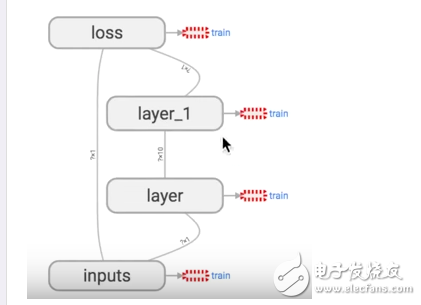
就是用 with tf.name_scope 定义各个框架，注意看代码注释中的区别：

import tensorflow as tf

def add_layer（inputs， in_size， out_size， activation_function=None）：

# add one more layer and return the output of this layer

# 区别：大框架，定义层 layer，里面有 小部件

with tf.name_scope（‘layer’）：

# 区别：小部件

with tf.name_scope（‘weights’）：

Weights = tf.Variable（tf.random_normal（［in_size， out_size］）， name=‘W’）

with tf.name_scope（‘biases’）：

biases = tf.Variable（tf.zeros（［1， out_size］） + 0.1， name=‘b’）

with tf.name_scope（‘Wx_plus_b’）：

Wx_plus_b = tf.add（tf.matmul（inputs， Weights）， biases）

if activation_function is None：

outputs = Wx_plus_b

else：

outputs = activation_function（Wx_plus_b， ）

return outputs

# define placeholder for inputs to network

# 区别：大框架，里面有 inputs x，y

with tf.name_scope（‘inputs’）：

xs = tf.placeholder（tf.float32， ［None， 1］， name=‘x_input’）

ys = tf.placeholder（tf.float32， ［None， 1］， name=‘y_input’）

# add hidden layer

l1 = add_layer（xs， 1， 10， activation_function=tf.nn.relu）

# add output layer

prediction = add_layer（l1， 10， 1， activation_function=None）

# the error between prediciton and real data

# 区别：定义框架 loss

with tf.name_scope（‘loss’）：

loss = tf.reduce_mean（tf.reduce_sum（tf.square（ys - prediction），

reduction_indices=［1］））

# 区别：定义框架 train

with tf.name_scope（‘train’）：

train_step = tf.train.GradientDescentOptimizer（0.1）.minimize（loss）

sess = tf.Session（）

# 区别：sess.graph 把所有框架加载到一个文件中放到文件夹“logs/”里

# 接着打开terminal，进入你存放的文件夹地址上一层，运行命令 tensorboard --logdir=‘logs/’

# 会返回一个地址，然后用浏览器打开这个地址，在 graph 标签栏下打开

writer = tf.train.SummaryWriter（“logs/”， sess.graph）

# important step

sess.run（tf.initialize_all_variables（））

运行完上面代码后，打开 terminal，进入你存放的文件夹地址上一层，运行命令 tensorboard --logdir=‘logs/’ 后会返回一个地址，然后用浏览器打开这个地址，点击 graph 标签栏下就可以看到流程图了

 

6. 保存和加载训练好了一个神经网络后，可以保存起来下次使用时再次加载：import tensorflow as tf

import numpy as np

## Save to file

# remember to define the same dtype and shape when restore

W = tf.Variable（［［1，2，3］，［3，4，5］］， dtype=tf.float32， name=‘weights’）

b = tf.Variable（［［1，2，3］］， dtype=tf.float32， name=‘biases’）

init= tf.initialize_all_variables（）

saver = tf.train.Saver（）

# 用 saver 将所有的 variable 保存到定义的路径

with tf.Session（） as sess：

sess.run（init）

save_path = saver.save（sess， “my_net/save_net.ckpt”）

print（“Save to path： ”， save_path）

################################################

# restore variables

# redefine the same shape and same type for your variables

W = tf.Variable（np.arange（6）.reshape（（2， 3））， dtype=tf.float32， name=“weights”）

b = tf.Variable（np.arange（3）.reshape（（1， 3））， dtype=tf.float32， name=“biases”）

# not need init step

saver = tf.train.Saver（）

# 用 saver 从路径中将 save_net.ckpt 保存的 W 和 b restore 进来

with tf.Session（） as sess：

saver.restore（sess， “my_net/save_net.ckpt”）

print（“weights：”， sess.run（W））

print（“biases：”， sess.run（b））

 

#p##e#

        简单搭建自己的神经网络

1. 模型阐述

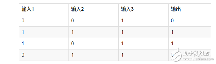
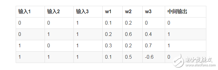
假设我们有下面的一组数据

 

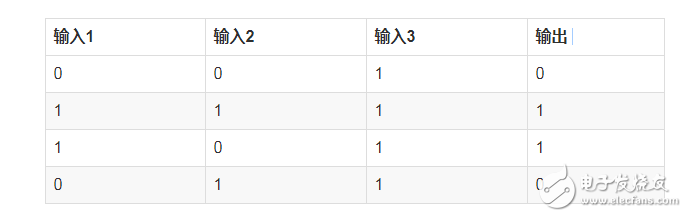
对于上面的表格，我们可以找出其中的一个规律是：

输入的第一列和输出相同

那对于输入有3列，每列有0和1两个值，那可能的排列有（2^3=8）种，但是此处只有4种，那么在有限的数据情况下，我们应该怎么预测其他结果呢？

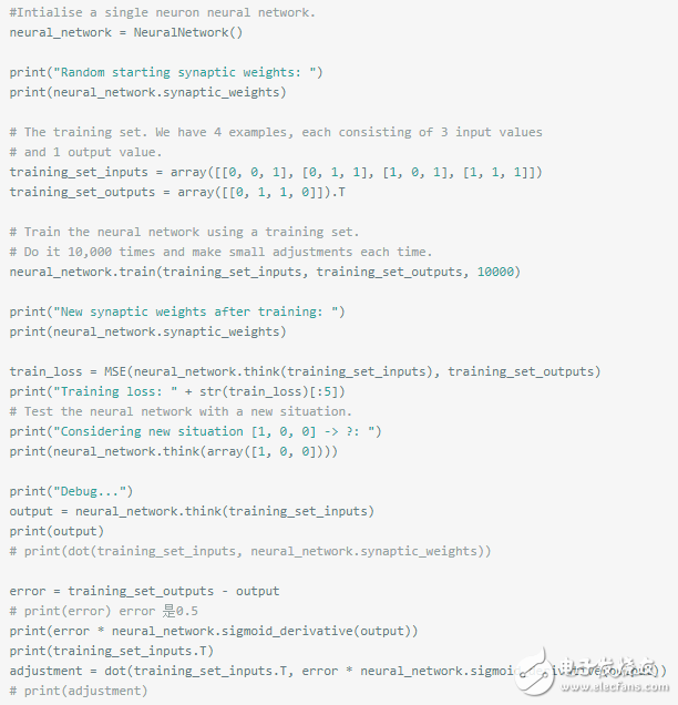
看代码：

%matplotlib inline

%config InlineBackend.figure_format = ‘retina’

from numpy import exp， array， random， dot

class NeuralNetwork（）：

def __init__（self）：

# Seed the random number generator， so it generates the same numbers

# every time the program runs.

random.seed（1）

# We model a single neuron， with 3 input connections and 1 output connection.

# We assign random weights to a 3 x 1 matrix， with values in the range -1 to 1

# and mean 0.

self.synaptic_weights = 2 * random.random（（3， 1）） - 1

self.sigmoid_derivative = self.__sigmoid_derivative

# The Sigmoid function， which describes an S shaped curve.

# We pass the weighted sum of the inputs through this function to

# normalise them between 0 and 1.

def __sigmoid（self， x）：

return 1 / （1 + exp（-x））

# The derivative of the Sigmoid function.

# This is the gradient of the Sigmoid curve.

# It indicates how confident we are about the existing weight.

def __sigmoid_derivative（self， x）：

return x * （1 - x）

# We train the neural network through a process of trial and error.

# Adjusting the synaptic weights each time.

def train（self， training_set_inputs， training_set_outputs， number_of_training_iterations）：

for iteration in range（number_of_training_iterations）：

# Pass the training set through our neural network （a single neuron）。

output = self.think（training_set_inputs）

# Calculate the error （The difference between the desired output

# and the predicted output）。

error = training_set_outputs - output

# Multiply the error by the input and again by the gradient of the Sigmoid curve.

# This means less confident weights are adjusted more.

# This means inputs， which are zero， do not cause changes to the weights.

adjustment = dot（training_set_inputs.T， error * self.__sigmoid_derivative（output））

# Adjust the weights.

self.synaptic_weights += adjustment

# The neural network thinks.

def think（self， inputs）：

# Pass inputs through our neural network （our single neuron）。

return self.__sigmoid（dot（inputs， self.synaptic_weights））

#Intialise a single neuron neural network.

neural_network = NeuralNetwork（）

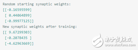
print（“Random starting synaptic weights： ”）

print（neural_network.synaptic_weights）

# The training set. We have 4 examples， each consisting of 3 input values# and 1 output value.

training_set_inputs = array（［［0， 0， 1］， ［1， 1， 1］， ［1， 0， 1］， ［0， 1， 1］］）

training_set_outputs = array（［［0， 1， 1， 0］］）.T

# Train the neural network using a training set.# Do it 10，000 times and make small adjustments each time.

neural_network.train（training_set_inputs， training_set_outputs， 10000）

print（“New synaptic weights after training： ”）

print（neural_network.synaptic_weights）

# Test the neural network with a new situation.

print（“Considering new situation ［1， 0， 0］ -》 ？： ”）

print（neural_network.think（array（［1， 0， 0］）））

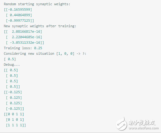
Random starting synaptic weights： ［［-0.16595599］

［ 0.44064899］

［-0.99977125］］

New synaptic weights after training： ［［ 9.67299303］

［-0.2078435 ］

［-4.62963669］］

Considering new situation ［1， 0， 0］ -》 ？： ［ 0.99993704］

以上代码来自：https://github.com/llSourcell/Make_a_neural_network

现在我们来分析下具体的过程：

第一个我们需要注意的是sigmoid function，其图如下：

import matplotlib.pyplot as pltimport numpy as np

def sigmoid（x）：

a = ［］

for item in x：

a.append（1/（1+np.exp（-item）））

return a

x = np.arange（-6.， 6.， 0.2）

sig = sigmoid（x）

plt.plot（x，sig）

plt.grid（）

plt.show（）

 

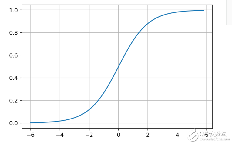
我们可以看到sigmoid函数将输入转换到了0-1之间的值，而sigmoid函数的导数是：

def __sigmoid_derivative（self， y）：

return y * （1 - y）

其具体的含义看图：

def sigmoid_derivative（x）：

y = 1/（1+np.exp（-x））

return y * （1-y）

def derivative（point）：

dx = np.arange（-0.5，0.5，0.1）

slope = sigmoid_derivative（point）

return ［point+dx，slope * dx + 1/（1+np.exp（-point））］

x = np.arange（-6.， 6.， 0.1）

sig = sigmoid（x）

point1 = 2

slope1 = sigmoid_derivative（point1）

plt.plot（x，sig）

x1，y1 = derivative（point1）

plt.plot（x1，y1，linewidth=5）

x2，y2 = derivative（0）

plt.plot（x2，y2，linewidth=5）

x3，y3 = derivative（-4）

plt.plot（x3，y3，linewidth=5）

plt.grid（）

plt.show（）

 

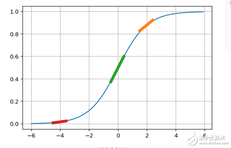
现在我们来根据图解释下实际的含义：

1. 首先输出是0到1之间的值，我们可以将其认为是一个可信度，0不可信，1完全可信

2. 当输入是0的时候，输出是0.5，什么意思呢？意思是输出模棱两可

基于以上两点，我们来看下上面函数的中的一个计算过程：

adjustment = dot（training_set_inputs.T， error * self.__sigmoid_derivative（output））

这个调整值的含义我们就知道了，当输出接近0和1时候，我们已经预测的挺准了，此时调整就基本接近于0了

而当输出为0.5左右的时候，说明预测完全是瞎猜，我们就需要快速调整，因此此时的导数也是最大的，即上图的绿色曲线，其斜度也是最大的

基于上面的一个讨论，我们还可以有下面的一个结论：

1. 当输入是1，输出是0，我们需要不断减小 weight 的值，这样子输出才会是很小，sigmoid输出才会是0

2. 当输入是1，输出是1，我们需要不断增大 weight 的值，这样子输出才会是很大，sigmoid输出才会是1

这时候我们再来看下最初的数据，

 

我们可以断定输入1的weight值会变大，而输入2，3的weight值会变小。

根据之前训练出来的结果也支持了我们的推断：

2. 扩展

我们来将上面的问题稍微复杂下，假设我们的输入如下：

 

此处我们只是改变一个值，此时我们再次训练呢？

我们观察上面的数据，好像很难再像最初一样直接观察出 输出1 == 输出 的这种简单的关系了，我们要稍微深入的观察下了

· 首先输入3都是1，看起来对输出没什么影响

· 接着观察输入1和输入2，似乎只要两者不同，输出就是1

基于上面的观察，我们似乎找不到像输出1 == 输出这种 one-to-one 的关系了，我们有什么办法呢？

这个时候，就需要引入 hidden layer，如下表格：

 

此时我们得到中的中间输入和最后输出就还是原来的一个 输出1 == 输出 关系了。

上面介绍的这种方法就是深度学习的最简单的形式

深度学习就是通过增加层次，不断去放大输入和输出之间的关系，到最后，我们可以从复杂的初看起来毫不相干的数据中，找到一个能一眼就看出来的关系

此处我们还是用之前的网络来训练

 

此处我们训练可以发现，此处的误差基本就是0.25，然后预测基本不可信。0.5什么鬼！

由数据可以看到此处的weight都已经非常非常小了，然后斜率是0.5，

由上面打印出来的数据，已经达到平衡，adjustment都是0了，不会再次调整了。

由此可以看出，简单的一层网络已经不能再精准的预测了，只能增加复杂度了。

下面我们来加一层再来看下：

class TwoLayerNeuralNetwork（object）：

def __init__（self， input_nodes， hidden_nodes， output_nodes， learning_rate）：

# Set number of nodes in input， hidden and output layers.

self.input_nodes = input_nodes

self.hidden_nodes = hidden_nodes

self.output_nodes = output_nodes

np.random.seed（1）

# Initialize weights

self.weights_0_1 = np.random.normal（0.0， self.hidden_nodes**-0.5，

（self.input_nodes， self.hidden_nodes）） # n * 2

self.weights_1_2 = np.random.normal（0.0， self.output_nodes**-0.5，

（self.hidden_nodes， self.output_nodes）） # 2 * 1

self.lr = learning_rate

#### Set this to your implemented sigmoid function ####

# Activation function is the sigmoid function

self.activation_function = self.__sigmoid

def __sigmoid（self， x）：

return 1 / （1 + np.exp（-x））

def __sigmoid_derivative（self， x）：

return x * （1 - x）

def train（self， inputs_list， targets_list）：

# Convert inputs list to 2d array

inputs = np.array（inputs_list，ndmin=2） # 1 * n

layer_0 = inputs

targets = np.array（targets_list，ndmin=2） # 1 * 1

#### Implement the forward pass here ####

### Forward pass ###

layer_1 = self.activation_function（layer_0.dot（self.weights_0_1）） # 1 * 2

layer_2 = self.activation_function（layer_1.dot（self.weights_1_2）） # 1 * 1

#### Implement the backward pass here ####

### Backward pass ###

# TODO： Output error

layer_2_error = targets - layer_2

layer_2_delta = layer_2_error * self.__sigmoid_derivative（layer_2）# y = x so f‘（h） = 1

layer_1_error = layer_2_delta.dot（self.weights_1_2.T）

layer_1_delta = layer_1_error * self.__sigmoid_derivative（layer_1）

# TODO： Update the weights

self.weights_1_2 += self.lr * layer_1.T.dot（layer_2_delta） # update hidden-to-output weights with gradient descent step

self.weights_0_1 += self.lr * layer_0.T.dot（layer_1_delta） # update input-to-hidden weights with gradient descent step

def run（self， inputs_list）：

# Run a forward pass through the network

inputs = np.array（inputs_list，ndmin=2）

#### Implement the forward pass here ####

layer_1 = self.activation_function（inputs.dot（self.weights_0_1）） # 1 * 2

layer_2 = self.activation_function（layer_1.dot（self.weights_1_2）） # 1 * 1

return layer_2def MSE（y， Y）：

return np.mean（（y-Y）**2）

# import sys

training_set_inputs = array（［［0， 0， 1］， ［0， 1， 1］， ［1， 0， 1］， ［1， 1， 1］］）

training_set_outputs = array（［［0， 1， 1， 0］］）.T

### Set the hyperparameters here ###

epochs = 20000

learning_rate = 0.1

hidden_nodes = 4

output_nodes = 1

N_i = 3

network = TwoLayerNeuralNetwork（N_i， hidden_nodes， output_nodes， learning_rate）

losses = {’train‘：［］}for e in range（epochs）：

# Go through a random batch of 128 records from the training data set

for record， target in zip（training_set_inputs，

training_set_outputs）：# print（target）

network.train（record， target）

train_loss = MSE（network.run（training_set_inputs）， training_set_outputs）

sys.stdout.write（“ Progress： ” + str（100 * e/float（epochs））［：4］

+ “% 。。。 Training loss： ” + str（train_loss）［：7］）

losses［’train‘］.append（train_loss）

print（“ ”）

print（“After train，layer_0_1： ”）

print（network.weights_0_1）

print（“After train，layer_1_2： ”）

print（network.weights_1_2）# Test the neural network with a new situation.

print（“Considering new situation ［1， 0， 0］ -》 ？： ”）

print（network.run（array（［1， 0， 0］）））

Progress： 99.9% 。。。 Training loss： 0.00078

After train，layer_0_1：

［［ 4.4375838 -3.87815184 1.74047905 -5.12726884］

［ 4.43114847 -3.87644617 1.71905492 -5.10688387］

［-6.80858063 0.76685389 1.89614363 1.61202043］］

After train，layer_1_2：

［［-9.21973137］

［-3.84985864］

［ 4.75257888］

［-6.36994226］］

Considering new situation ［1， 0， 0］ -》 ？：

［［ 0.00557239］］

layer_1=network.activation_function（training_set_inputs.dot（network.weights_0_1））

print（layer_1）

layer_2 = network.activation_function（layer_1.dot（network.weights_1_2））

print（layer_2）

［［ 2.20482250e-01 9.33639853e-01 6.30402293e-01 6.24775766e-02］

［ 1.77659862e-02 9.99702482e-01 8.64290928e-01 9.26611880e-01］

［ 6.94975743e-01 8.90040645e-02 8.51261229e-01 2.06917379e-04］

［ 1.27171786e-01 9.58904341e-01 9.55296949e-01 3.77322214e-02］］

［［ 0.02374213］

［ 0.97285992］

［ 0.97468116］

［ 0.02714965］］

最后总结：我们发现在扩展中，我们只是简单的改变了两个输入值，此时再次用一层神经网络已经难以预测出正确的数据了，此时我们只能通过将神经网络变深，这个过程其实就是再去深度挖掘数据之间关系的过程，此时我们的2层神经网络相比较1层就好多了。